

8.3 One-Dimensional Arrays of MCCs
331
−
L
R
i L,i (t 0 ) −
k∈N i
1
R ik
(ϕ M 0,k − ϕ M 0,i )
for any t ≥ t 0 and i = 1, 2, . . . , N.
Remark 8.2 From the proof of Property 8.2 it is seen that Q i (w c ) (i = 1, 2, . . . , N)
provide N invariants of motion for the dynamics of the NMCC in the (v, i)-domain.
8.3.1 Adimensional Normal Form of State Equations in the
Flux-Charge Domain
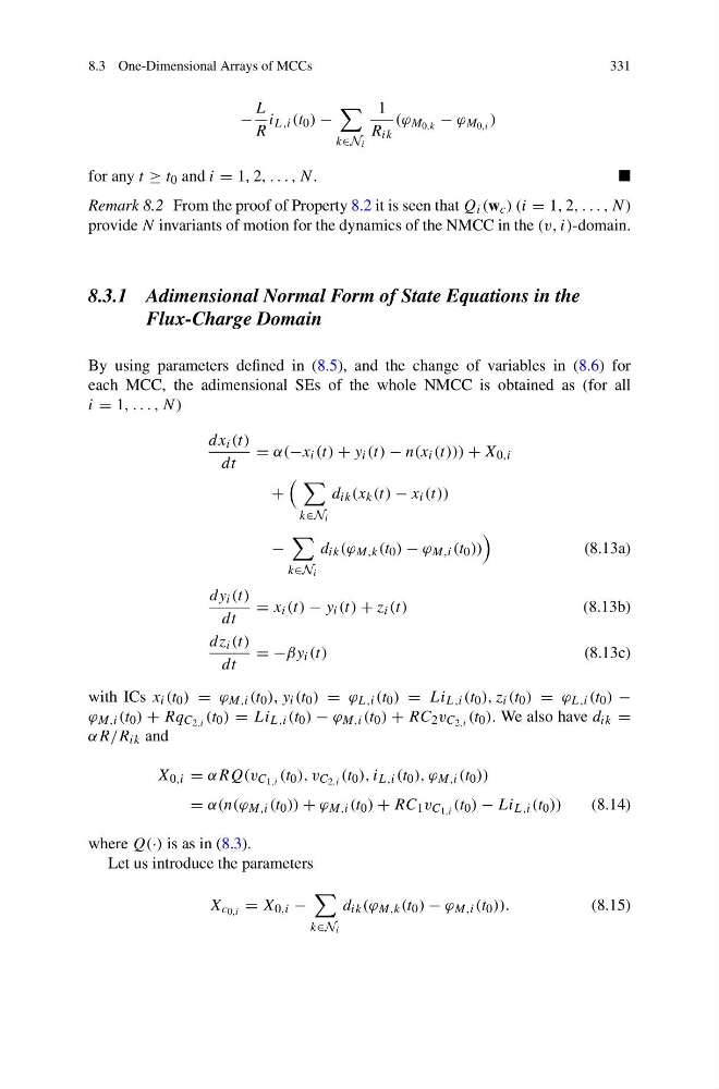
By using parameters defined in (8.5), and the change of variables in (8.6) for
each MCC, the adimensional SEs of the whole NMCC is obtained as (for all
i = 1, . . . , N)
dx i (t)
dt
= α(−x i (t) + y i (t) − n(x i (t))) + X 0,i
+
k∈N i
d ik (x k (t) − x i (t))
−
k∈N i
d ik (ϕ M,k (t 0 ) − ϕ M,i (t 0 ))
(8.13a)
dy i (t)
dt
= x i (t) − y i (t) + z i (t)
(8.13b)
dz i (t)
dt
= −βy i (t)
(8.13c)
with ICs x i (t 0 ) = ϕ M,i (t 0 ), y i (t 0 ) = ϕ L,i (t 0 ) = Li L,i (t 0 ), z i (t 0 ) = ϕ L,i (t 0 ) −
ϕ M,i (t 0 ) + Rq C 2,i (t 0 ) = Li L,i (t 0 ) − ϕ M,i (t 0 ) + RC 2 v C 2,i (t 0 ). We also have d ik =
αR/R ik and
X 0,i = αRQ(v C 1,i (t 0 ), v C 2,i (t 0 ), i L,i (t 0 ), ϕ M,i (t 0 ))
= α(n(ϕ M,i (t 0 )) + ϕ M,i (t 0 ) + RC 1 v C 1,i (t 0 ) − Li L,i (t 0 ))
(8.14)
where Q(·) is as in (8.3).
Let us introduce the parameters
X c 0,i = X 0,i −
k∈N i
d ik (ϕ M,k (t 0 ) − ϕ M,i (t 0 )).
(8.15)
331
−
L
R
i L,i (t 0 ) −
k∈N i
1
R ik
(ϕ M 0,k − ϕ M 0,i )
for any t ≥ t 0 and i = 1, 2, . . . , N.
Remark 8.2 From the proof of Property 8.2 it is seen that Q i (w c ) (i = 1, 2, . . . , N)
provide N invariants of motion for the dynamics of the NMCC in the (v, i)-domain.
8.3.1 Adimensional Normal Form of State Equations in the
Flux-Charge Domain
By using parameters defined in (8.5), and the change of variables in (8.6) for
each MCC, the adimensional SEs of the whole NMCC is obtained as (for all
i = 1, . . . , N)
dx i (t)
dt
= α(−x i (t) + y i (t) − n(x i (t))) + X 0,i
+
k∈N i
d ik (x k (t) − x i (t))
−
k∈N i
d ik (ϕ M,k (t 0 ) − ϕ M,i (t 0 ))
(8.13a)
dy i (t)
dt
= x i (t) − y i (t) + z i (t)
(8.13b)
dz i (t)
dt
= −βy i (t)
(8.13c)
with ICs x i (t 0 ) = ϕ M,i (t 0 ), y i (t 0 ) = ϕ L,i (t 0 ) = Li L,i (t 0 ), z i (t 0 ) = ϕ L,i (t 0 ) −
ϕ M,i (t 0 ) + Rq C 2,i (t 0 ) = Li L,i (t 0 ) − ϕ M,i (t 0 ) + RC 2 v C 2,i (t 0 ). We also have d ik =
αR/R ik and
X 0,i = αRQ(v C 1,i (t 0 ), v C 2,i (t 0 ), i L,i (t 0 ), ϕ M,i (t 0 ))
= α(n(ϕ M,i (t 0 )) + ϕ M,i (t 0 ) + RC 1 v C 1,i (t 0 ) − Li L,i (t 0 ))
(8.14)
where Q(·) is as in (8.3).
Let us introduce the parameters
X c 0,i = X 0,i −
k∈N i
d ik (ϕ M,k (t 0 ) − ϕ M,i (t 0 )).
(8.15)