

306
7 Pulse Programming of Memristor Circuits
H =
0 −1
1 R
and
u(t) =
q a (t; t 0 )
−ϕ e (t; t 0 ) + Rq a (t; t 0 )
where q a (t; t 0 ) =
t
t 0
a(τ )dτ and ϕ e (t; t 0 ) =
t
t 0
e(τ )dτ .
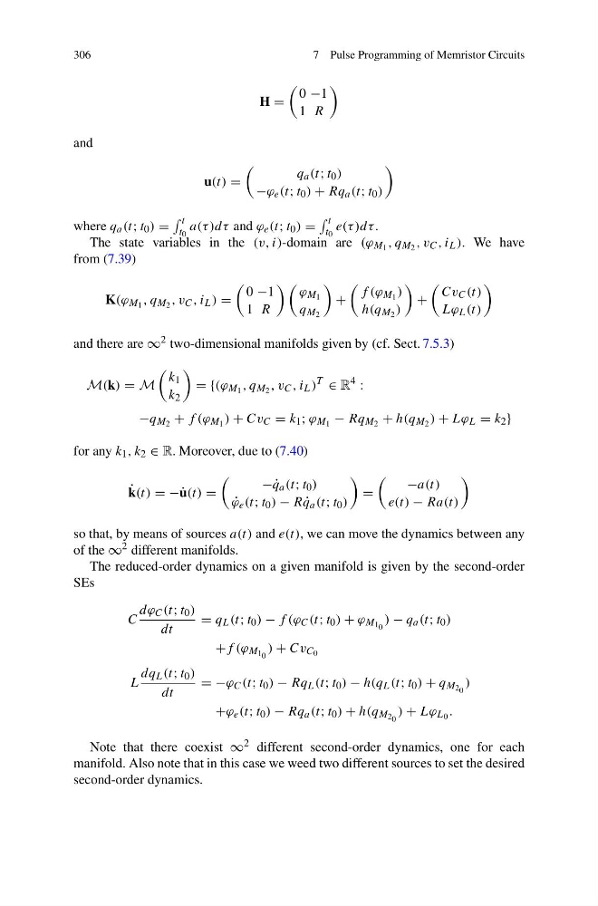
The state variables in the (v, i)-domain are (ϕ M 1 , q M 2 , v C , i L ). We have
from (7.39)
K(ϕ M 1 , q M 2 , v C , i L ) =
0 −1
1 R
ϕ M 1
q M 2
+
f (ϕ M 1 )
h(q M 2 )
+
Cv C (t)
Lϕ L (t)
and there are ∞ 2 two-dimensional manifolds given by (cf. Sect. 7.5.3)
M(k) = M
k 1
k 2
= {(ϕ M 1 , q M 2 , v C , i L )
T
∈ R
4
:
−q M 2 + f (ϕ M 1 ) + Cv C = k 1 ; ϕ M 1 − Rq M 2 + h(q M 2 ) + Lϕ L = k 2 }
for any k 1 , k 2 ∈ R. Moreover, due to (7.40)
˙
k(t) = −˙ u(t) =
− ˙
q a (t; t 0 )
˙
ϕ e (t; t 0 ) − R ˙
q a (t; t 0 )
=
−a(t)
e(t) − Ra(t)
so that, by means of sources a(t) and e(t), we can move the dynamics between any
of the ∞ 2 different manifolds.
The reduced-order dynamics on a given manifold is given by the second-order
SEs
C
dϕ C (t; t 0 )
dt
= q L (t; t 0 ) − f (ϕ C (t; t 0 ) + ϕ M 1 0 ) − q a (t; t 0 )
+f (ϕ M 1 0 ) + Cv C 0
L
dq L (t; t 0 )
dt
= −ϕ C (t; t 0 ) − Rq L (t; t 0 ) − h(q L (t; t 0 ) + q M 2 0 )
+ϕ e (t; t 0 ) − Rq a (t; t 0 ) + h(q M 2 0 ) + Lϕ L 0 .
Note that there coexist ∞ 2 different second-order dynamics, one for each
manifold. Also note that in this case we weed two different sources to set the desired
second-order dynamics.
7 Pulse Programming of Memristor Circuits
H =
0 −1
1 R
and
u(t) =
q a (t; t 0 )
−ϕ e (t; t 0 ) + Rq a (t; t 0 )
where q a (t; t 0 ) =
t
t 0
a(τ )dτ and ϕ e (t; t 0 ) =
t
t 0
e(τ )dτ .
The state variables in the (v, i)-domain are (ϕ M 1 , q M 2 , v C , i L ). We have
from (7.39)
K(ϕ M 1 , q M 2 , v C , i L ) =
0 −1
1 R
ϕ M 1
q M 2
+
f (ϕ M 1 )
h(q M 2 )
+
Cv C (t)
Lϕ L (t)
and there are ∞ 2 two-dimensional manifolds given by (cf. Sect. 7.5.3)
M(k) = M
k 1
k 2
= {(ϕ M 1 , q M 2 , v C , i L )
T
∈ R
4
:
−q M 2 + f (ϕ M 1 ) + Cv C = k 1 ; ϕ M 1 − Rq M 2 + h(q M 2 ) + Lϕ L = k 2 }
for any k 1 , k 2 ∈ R. Moreover, due to (7.40)
˙
k(t) = −˙ u(t) =
− ˙
q a (t; t 0 )
˙
ϕ e (t; t 0 ) − R ˙
q a (t; t 0 )
=
−a(t)
e(t) − Ra(t)
so that, by means of sources a(t) and e(t), we can move the dynamics between any
of the ∞ 2 different manifolds.
The reduced-order dynamics on a given manifold is given by the second-order
SEs
C
dϕ C (t; t 0 )
dt
= q L (t; t 0 ) − f (ϕ C (t; t 0 ) + ϕ M 1 0 ) − q a (t; t 0 )
+f (ϕ M 1 0 ) + Cv C 0
L
dq L (t; t 0 )
dt
= −ϕ C (t; t 0 ) − Rq L (t; t 0 ) − h(q L (t; t 0 ) + q M 2 0 )
+ϕ e (t; t 0 ) − Rq a (t; t 0 ) + h(q M 2 0 ) + Lϕ L 0 .
Note that there coexist ∞ 2 different second-order dynamics, one for each
manifold. Also note that in this case we weed two different sources to set the desired
second-order dynamics.