

300
7 Pulse Programming of Memristor Circuits
f (ϕ M )
q M0
ϕ M0 q M (t; t 0 )
ϕ M (t; t 0 )
q C1 0
ϕ C1 (t; t 0 )
C 1
q C1 (t; t 0 )
D
ϕ
M
q C2 0
C 2
ϕ C2 (t; t 0 ) = ϕ γC (t; t 0 )
ϕ γM (t; t 0 )
D
ϕ
C
R
r
ϕ e (t; t 0 )
q a (t; t 0 )
N R
q γM (t; t 0 )
q γC (t; t 0 )
ϕ λL (t; t 0 )
q λL (t; t 0 )
ϕ L0
L
D
q
L
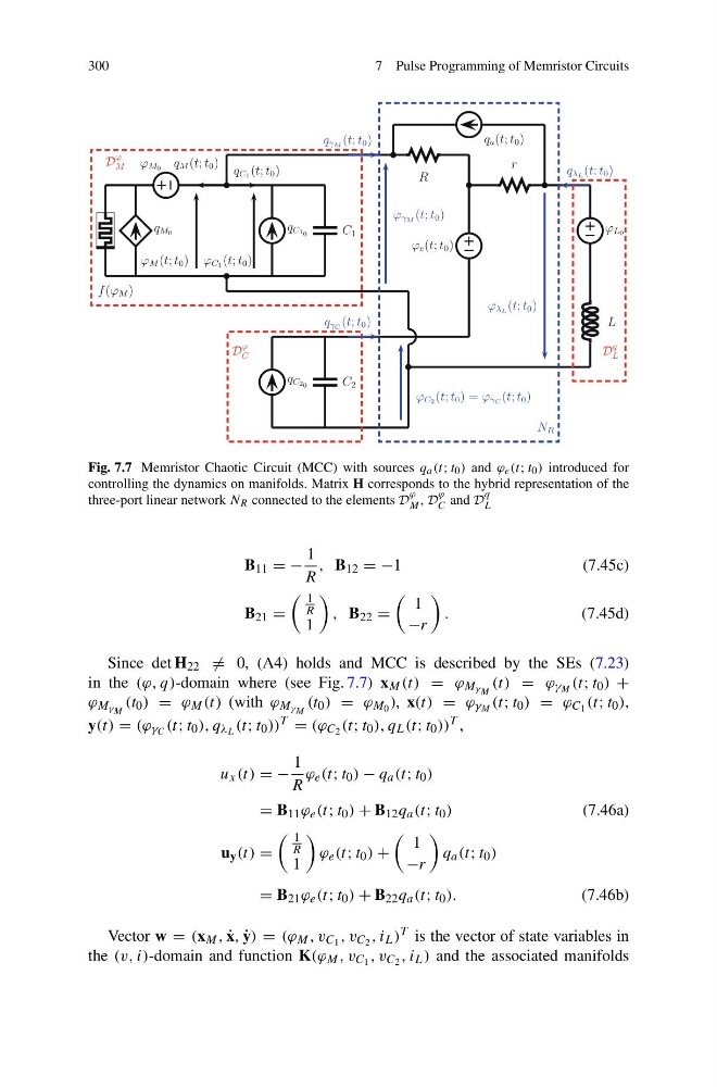
Fig. 7.7 Memristor Chaotic Circuit (MCC) with sources q a (t; t 0 ) and ϕ e (t; t 0 ) introduced for
controlling the dynamics on manifolds. Matrix H corresponds to the hybrid representation of the
three-port linear network N R connected to the elements D
ϕ
M , D
ϕ
C and D
q
L
B 11 = −
1
R
, B 12 = −1
(7.45c)
B 21 =
1
R
1
, B 22 =
1
−r
.
(7.45d)
Since det H 22 = 0, (A4) holds and MCC is described by the SEs (7.23)
in the (ϕ, q)-domain where (see Fig. 7.7) x M (t) = ϕ M γ M (t) = ϕ γ M (t; t 0 ) +
ϕ M γ M (t 0 ) = ϕ M (t) (with ϕ M γ M (t 0 ) = ϕ M 0 ), x(t) = ϕ γ M (t; t 0 ) = ϕ C 1 (t; t 0 ),
y(t) = (ϕ γ C (t; t 0 ), q λ L (t; t 0 )) T = (ϕ C 2 (t; t 0 ), q L (t; t 0 )) T ,
u x (t) = −
1
R
ϕ e (t; t 0 ) − q a (t; t 0 )
= B 11 ϕ e (t; t 0 ) + B 12 q a (t; t 0 )
(7.46a)
u y (t) =
1
R
1
ϕ e (t; t 0 ) +
1
−r
q a (t; t 0 )
= B 21 ϕ e (t; t 0 ) + B 22 q a (t; t 0 ).
(7.46b)
Vector w = (x M , ˙
x, ˙
y) = (ϕ M , v C 1 , v C 2 , i L ) T is the vector of state variables in
the (v, i)-domain and function K(ϕ M , v C 1 , v C 2 , i L ) and the associated manifolds
7 Pulse Programming of Memristor Circuits
f (ϕ M )
q M0
ϕ M0 q M (t; t 0 )
ϕ M (t; t 0 )
q C1 0
ϕ C1 (t; t 0 )
C 1
q C1 (t; t 0 )
D
ϕ
M
q C2 0
C 2
ϕ C2 (t; t 0 ) = ϕ γC (t; t 0 )
ϕ γM (t; t 0 )
D
ϕ
C
R
r
ϕ e (t; t 0 )
q a (t; t 0 )
N R
q γM (t; t 0 )
q γC (t; t 0 )
ϕ λL (t; t 0 )
q λL (t; t 0 )
ϕ L0
L
D
q
L
Fig. 7.7 Memristor Chaotic Circuit (MCC) with sources q a (t; t 0 ) and ϕ e (t; t 0 ) introduced for
controlling the dynamics on manifolds. Matrix H corresponds to the hybrid representation of the
three-port linear network N R connected to the elements D
ϕ
M , D
ϕ
C and D
q
L
B 11 = −
1
R
, B 12 = −1
(7.45c)
B 21 =
1
R
1
, B 22 =
1
−r
.
(7.45d)
Since det H 22 = 0, (A4) holds and MCC is described by the SEs (7.23)
in the (ϕ, q)-domain where (see Fig. 7.7) x M (t) = ϕ M γ M (t) = ϕ γ M (t; t 0 ) +
ϕ M γ M (t 0 ) = ϕ M (t) (with ϕ M γ M (t 0 ) = ϕ M 0 ), x(t) = ϕ γ M (t; t 0 ) = ϕ C 1 (t; t 0 ),
y(t) = (ϕ γ C (t; t 0 ), q λ L (t; t 0 )) T = (ϕ C 2 (t; t 0 ), q L (t; t 0 )) T ,
u x (t) = −
1
R
ϕ e (t; t 0 ) − q a (t; t 0 )
= B 11 ϕ e (t; t 0 ) + B 12 q a (t; t 0 )
(7.46a)
u y (t) =
1
R
1
ϕ e (t; t 0 ) +
1
−r
q a (t; t 0 )
= B 21 ϕ e (t; t 0 ) + B 22 q a (t; t 0 ).
(7.46b)
Vector w = (x M , ˙
x, ˙
y) = (ϕ M , v C 1 , v C 2 , i L ) T is the vector of state variables in
the (v, i)-domain and function K(ϕ M , v C 1 , v C 2 , i L ) and the associated manifolds