

6.2 Second-Order Memristor Oscillators
245
C
d
dt
ϕ C (t; t 0 ) = −q L (t; t 0 ) + q C 0
(6.29a)
L
d
dt
q L (t; t 0 ) = ϕ C (t; t 0 ) − h(q L (t; t 0 ) + q M 0 ) + h(q M 0 ) + ϕ L 0
(6.29b)
ϕ C (t 0 ; t 0 ) = 0
(6.29c)
q L (t 0 ; t 0 ) = 0.
(6.29d)
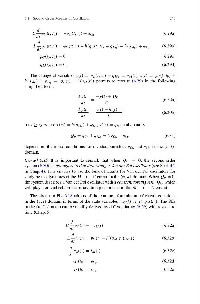
The change of variables y(t) = q L (t; t 0 ) + q M 0 = q M (t), x(t) = ϕ C (t; t 0 ) +
h(q M 0 ) + ϕ L 0 = ϕ L (t) + h(q M (t)) permits to rewrite (6.29) in the following
simplified form:
d x(t)
dt
=
−y(t) + Q 0
C
(6.30a)
d y(t)
dt
=
x(t) − h(y(t))
L
(6.30b)
for t ≥ t 0 , where x(t 0 ) = h(q M 0 ) + ϕ L 0 , y(t 0 ) = q M 0 and quantity
Q 0 = q C 0 + q M 0 = Cv C 0 + q M 0
(6.31)
depends on the initial conditions for the state variables v C 0 and q M 0 in the (v, i)domain.
Remark 6.15 It is important to remark that when Q 0 = 0, the second-order
system (6.30) is analogous to that describing a Van der Pol oscillator (see Sect. 4.2
in Chap. 4). This enables to use the bulk of results for Van der Pol oscillators for
studying the dynamics of the M −L−C circuit in the (ϕ, q)-domain. When Q 0 = 0,
the system describes a Van der Pol oscillator with a constant forcing term Q 0 , which
will play a crucial role in the bifurcation phenomena of the M − L − C circuit.
The circuit in Fig. 6.18 admits of the common formulation of circuit equations
in the (v, i)-domain in terms of the state variables (v C (t), i L (t), q M (t)). The SEs
in the (v, i)-domain can be readily derived by differentiating (6.29) with respect to
time (Chap. 5)
C
d
dt
v C (t) = −i L (t)
(6.32a)
L
d
dt
i L (t) = v C (t) − h
(q M (t))i M (t)
(6.32b)
d
dt
q M (t) = i M (t)
(6.32c)
v C (t 0 ) = v C 0
(6.32d)
i L (t 0 ) = i L 0
(6.32e)
245
C
d
dt
ϕ C (t; t 0 ) = −q L (t; t 0 ) + q C 0
(6.29a)
L
d
dt
q L (t; t 0 ) = ϕ C (t; t 0 ) − h(q L (t; t 0 ) + q M 0 ) + h(q M 0 ) + ϕ L 0
(6.29b)
ϕ C (t 0 ; t 0 ) = 0
(6.29c)
q L (t 0 ; t 0 ) = 0.
(6.29d)
The change of variables y(t) = q L (t; t 0 ) + q M 0 = q M (t), x(t) = ϕ C (t; t 0 ) +
h(q M 0 ) + ϕ L 0 = ϕ L (t) + h(q M (t)) permits to rewrite (6.29) in the following
simplified form:
d x(t)
dt
=
−y(t) + Q 0
C
(6.30a)
d y(t)
dt
=
x(t) − h(y(t))
L
(6.30b)
for t ≥ t 0 , where x(t 0 ) = h(q M 0 ) + ϕ L 0 , y(t 0 ) = q M 0 and quantity
Q 0 = q C 0 + q M 0 = Cv C 0 + q M 0
(6.31)
depends on the initial conditions for the state variables v C 0 and q M 0 in the (v, i)domain.
Remark 6.15 It is important to remark that when Q 0 = 0, the second-order
system (6.30) is analogous to that describing a Van der Pol oscillator (see Sect. 4.2
in Chap. 4). This enables to use the bulk of results for Van der Pol oscillators for
studying the dynamics of the M −L−C circuit in the (ϕ, q)-domain. When Q 0 = 0,
the system describes a Van der Pol oscillator with a constant forcing term Q 0 , which
will play a crucial role in the bifurcation phenomena of the M − L − C circuit.
The circuit in Fig. 6.18 admits of the common formulation of circuit equations
in the (v, i)-domain in terms of the state variables (v C (t), i L (t), q M (t)). The SEs
in the (v, i)-domain can be readily derived by differentiating (6.29) with respect to
time (Chap. 5)
C
d
dt
v C (t) = −i L (t)
(6.32a)
L
d
dt
i L (t) = v C (t) − h
(q M (t))i M (t)
(6.32b)
d
dt
q M (t) = i M (t)
(6.32c)
v C (t 0 ) = v C 0
(6.32d)
i L (t 0 ) = i L 0
(6.32e)