

236
6 Memristor Circuits: Invariant Manifolds, Coexisting Attractors, Extreme. . .
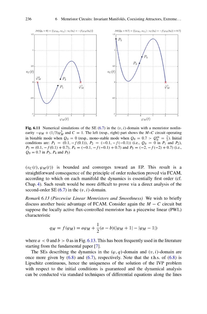
Fig. 6.11 Numerical simulations of the SE (6.7) in the (v, i)-domain with a memristor nonlinearity −ϕ M + (1/3)ϕ 3
M and C = 1. The left (resp., right) part shows the M–C circuit operating
in bistable mode when Q 0 = 0 (resp., mono-stable mode when Q 0 = 0.7 > Q sn
0 =
2
3 ). Initial
conditions are: P 1 = (0.1, −f (0.1)), P 2 = (−0.1, −f (−0.1)) (i.e., Q 0 = 0 in P 1 and P 2 ),
P 3 = (0.1, −f (0.1) + 0.7), P 4 = (−0.1, −f (−0.1) + 0.7) and P 5 = (−2, −f (−2) + 0.7) (i.e.,
Q 0 = 0.7 in P 3 , P 4 and P 5 )
(v C (t), ϕ M (t)) is bounded and converges toward an EP. This result is a
straightforward consequence of the principle of order reduction proved via FCAM,
according to which on each manifold the dynamics is essentially first order (cf.
Chap. 4). Such result would be more difficult to prove via a direct analysis of the
second-order SE (6.7) in the (v, i)-domain.
Remark 6.13 (Piecewise Linear Memristors and Smoothness) We wish to briefly
discuss another basic advantage of FCAM. Consider again the M − C circuit but
suppose the locally active flux-controlled memristor has a piecewise linear (PWL)
characteristic
q M = f (ϕ M ) = aϕ M +
1
2
(a − b)(|ϕ M + 1| − |ϕ M − 1|)
where a < 0 and b > 0 as in Fig. 6.13. This has been frequently used in the literature
starting from the fundamental paper [7].
The SEs describing the dynamics in the (ϕ, q)-domain and (v, i)-domain are
once more given by (6.8) and (6.7), respectively. Note that the r.h.s. of (6.8) is
Lipschitz continuous, hence the uniqueness of the solution of the IVP problem
with respect to the initial conditions is guaranteed and the dynamical analysis
can be conducted via standard techniques of differential equations along the lines
6 Memristor Circuits: Invariant Manifolds, Coexisting Attractors, Extreme. . .
Fig. 6.11 Numerical simulations of the SE (6.7) in the (v, i)-domain with a memristor nonlinearity −ϕ M + (1/3)ϕ 3
M and C = 1. The left (resp., right) part shows the M–C circuit operating
in bistable mode when Q 0 = 0 (resp., mono-stable mode when Q 0 = 0.7 > Q sn
0 =
2
3 ). Initial
conditions are: P 1 = (0.1, −f (0.1)), P 2 = (−0.1, −f (−0.1)) (i.e., Q 0 = 0 in P 1 and P 2 ),
P 3 = (0.1, −f (0.1) + 0.7), P 4 = (−0.1, −f (−0.1) + 0.7) and P 5 = (−2, −f (−2) + 0.7) (i.e.,
Q 0 = 0.7 in P 3 , P 4 and P 5 )
(v C (t), ϕ M (t)) is bounded and converges toward an EP. This result is a
straightforward consequence of the principle of order reduction proved via FCAM,
according to which on each manifold the dynamics is essentially first order (cf.
Chap. 4). Such result would be more difficult to prove via a direct analysis of the
second-order SE (6.7) in the (v, i)-domain.
Remark 6.13 (Piecewise Linear Memristors and Smoothness) We wish to briefly
discuss another basic advantage of FCAM. Consider again the M − C circuit but
suppose the locally active flux-controlled memristor has a piecewise linear (PWL)
characteristic
q M = f (ϕ M ) = aϕ M +
1
2
(a − b)(|ϕ M + 1| − |ϕ M − 1|)
where a < 0 and b > 0 as in Fig. 6.13. This has been frequently used in the literature
starting from the fundamental paper [7].
The SEs describing the dynamics in the (ϕ, q)-domain and (v, i)-domain are
once more given by (6.8) and (6.7), respectively. Note that the r.h.s. of (6.8) is
Lipschitz continuous, hence the uniqueness of the solution of the IVP problem
with respect to the initial conditions is guaranteed and the dynamical analysis
can be conducted via standard techniques of differential equations along the lines