

202
5 Flux-Charge Analysis Method of Memristor Circuits
⎧
⎨
⎩
Ai(t) = 0
Bv(t) = 0
(5.37)
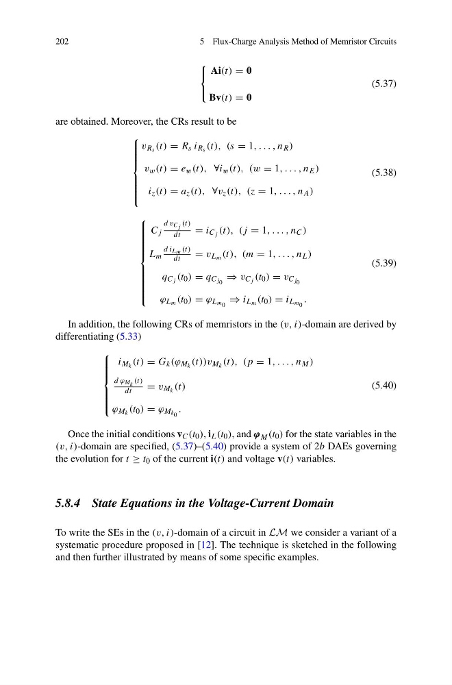
are obtained. Moreover, the CRs result to be
⎧
⎪ ⎪ ⎪ ⎪ ⎪ ⎨
⎪ ⎪ ⎪ ⎪ ⎪ ⎩
v R s (t) = R s i R s (t), (s = 1, . . . , n R )
v w (t) = e w (t), ∀i w (t), (w = 1, . . . , n E )
i z (t) = a z (t), ∀v z (t), (z = 1, . . . , n A )
(5.38)
⎧
⎪ ⎪ ⎪ ⎪ ⎪ ⎪ ⎪ ⎪ ⎨
⎪ ⎪ ⎪ ⎪ ⎪ ⎪ ⎪ ⎪ ⎩
C j
d v C j (t)
dt
= i C j (t), (j = 1, . . . , n C )
L m
d i Lm (t)
dt
= v L m (t), (m = 1, . . . , n L )
q C j (t 0 ) = q C j 0 ⇒ v C j (t 0 ) = v C j 0
ϕ L m (t 0 ) = ϕ L m 0 ⇒ i L m (t 0 ) = i L m 0 .
(5.39)
In addition, the following CRs of memristors in the (v, i)-domain are derived by
differentiating (5.33)
⎧
⎪ ⎪ ⎪ ⎪ ⎨
⎪ ⎪ ⎪ ⎪ ⎩
i M k (t) = G k (ϕ M k (t))v M k (t), (p = 1, . . . , n M )
d ϕ M k (t)
dt
= v M k (t)
ϕ M k (t 0 ) = ϕ M k 0 .
(5.40)
Once the initial conditions v C (t 0 ), i L (t 0 ), and ϕ M (t 0 ) for the state variables in the
(v, i)-domain are specified, (5.37)–(5.40) provide a system of 2b DAEs governing
the evolution for t ≥ t 0 of the current i(t) and voltage v(t) variables.
5.8.4 State Equations in the Voltage-Current Domain
To write the SEs in the (v, i)-domain of a circuit in LM we consider a variant of a
systematic procedure proposed in [12]. The technique is sketched in the following
and then further illustrated by means of some specific examples.
5 Flux-Charge Analysis Method of Memristor Circuits
⎧
⎨
⎩
Ai(t) = 0
Bv(t) = 0
(5.37)
are obtained. Moreover, the CRs result to be
⎧
⎪ ⎪ ⎪ ⎪ ⎪ ⎨
⎪ ⎪ ⎪ ⎪ ⎪ ⎩
v R s (t) = R s i R s (t), (s = 1, . . . , n R )
v w (t) = e w (t), ∀i w (t), (w = 1, . . . , n E )
i z (t) = a z (t), ∀v z (t), (z = 1, . . . , n A )
(5.38)
⎧
⎪ ⎪ ⎪ ⎪ ⎪ ⎪ ⎪ ⎪ ⎨
⎪ ⎪ ⎪ ⎪ ⎪ ⎪ ⎪ ⎪ ⎩
C j
d v C j (t)
dt
= i C j (t), (j = 1, . . . , n C )
L m
d i Lm (t)
dt
= v L m (t), (m = 1, . . . , n L )
q C j (t 0 ) = q C j 0 ⇒ v C j (t 0 ) = v C j 0
ϕ L m (t 0 ) = ϕ L m 0 ⇒ i L m (t 0 ) = i L m 0 .
(5.39)
In addition, the following CRs of memristors in the (v, i)-domain are derived by
differentiating (5.33)
⎧
⎪ ⎪ ⎪ ⎪ ⎨
⎪ ⎪ ⎪ ⎪ ⎩
i M k (t) = G k (ϕ M k (t))v M k (t), (p = 1, . . . , n M )
d ϕ M k (t)
dt
= v M k (t)
ϕ M k (t 0 ) = ϕ M k 0 .
(5.40)
Once the initial conditions v C (t 0 ), i L (t 0 ), and ϕ M (t 0 ) for the state variables in the
(v, i)-domain are specified, (5.37)–(5.40) provide a system of 2b DAEs governing
the evolution for t ≥ t 0 of the current i(t) and voltage v(t) variables.
5.8.4 State Equations in the Voltage-Current Domain
To write the SEs in the (v, i)-domain of a circuit in LM we consider a variant of a
systematic procedure proposed in [12]. The technique is sketched in the following
and then further illustrated by means of some specific examples.