

5.5 Flux-Charge Analysis Method (FCAM) for Class LM of Memristor Circuits
181
which no longer involves the initial charges q(t 0 ), but just expresses the constraints
on the incremental charges due to the circuit topology.
Similarly, the Kirchhoff Flux Law (KϕL) using the vector of incremental fluxes
ϕ(t; t 0 ) can be written as
Bϕ(t; t 0 ) = 0.
(5.22)
These laws will be referred to henceforth as conservation of incremental charge
and flux, respectively. It is known that these equations give in overall b independent
topological constraints on q(t; t 0 ) and ϕ(t; t 0 ) in the (ϕ, q)-domain (Chap. 3).
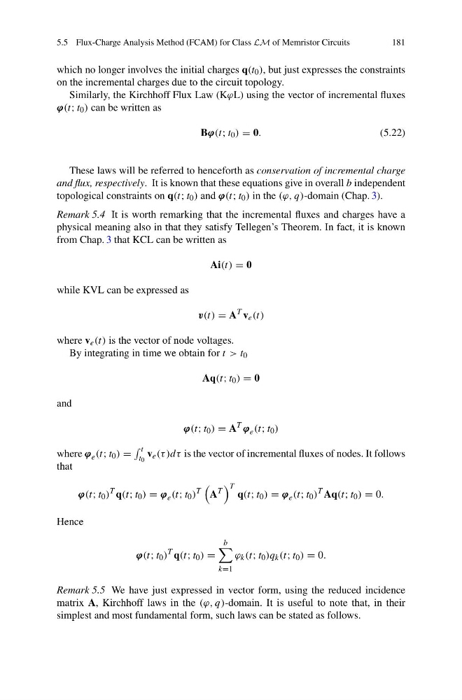
Remark 5.4 It is worth remarking that the incremental fluxes and charges have a
physical meaning also in that they satisfy Tellegen’s Theorem. In fact, it is known
from Chap. 3 that KCL can be written as
Ai(t) = 0
while KVL can be expressed as
v(t) = A
T v e (t)
where v e (t) is the vector of node voltages.
By integrating in time we obtain for t > t 0
Aq(t; t 0 ) = 0
and
ϕ(t; t 0 ) = A
T
ϕ e (t; t 0 )
where ϕ e (t; t 0 ) =
t
t 0
v e (τ )dτ is the vector of incremental fluxes of nodes. It follows
that
ϕ(t; t 0 )
T q(t; t 0 ) = ϕ e (t; t 0 )
T
A
T
T
q(t; t 0 ) = ϕ e (t; t 0 )
T Aq(t; t 0 ) = 0.
Hence
ϕ(t; t 0 )
T q(t; t 0 ) =
b
k=1
ϕ k (t; t 0 )q k (t; t 0 ) = 0.
Remark 5.5 We have just expressed in vector form, using the reduced incidence
matrix A, Kirchhoff laws in the (ϕ, q)-domain. It is useful to note that, in their
simplest and most fundamental form, such laws can be stated as follows.
181
which no longer involves the initial charges q(t 0 ), but just expresses the constraints
on the incremental charges due to the circuit topology.
Similarly, the Kirchhoff Flux Law (KϕL) using the vector of incremental fluxes
ϕ(t; t 0 ) can be written as
Bϕ(t; t 0 ) = 0.
(5.22)
These laws will be referred to henceforth as conservation of incremental charge
and flux, respectively. It is known that these equations give in overall b independent
topological constraints on q(t; t 0 ) and ϕ(t; t 0 ) in the (ϕ, q)-domain (Chap. 3).
Remark 5.4 It is worth remarking that the incremental fluxes and charges have a
physical meaning also in that they satisfy Tellegen’s Theorem. In fact, it is known
from Chap. 3 that KCL can be written as
Ai(t) = 0
while KVL can be expressed as
v(t) = A
T v e (t)
where v e (t) is the vector of node voltages.
By integrating in time we obtain for t > t 0
Aq(t; t 0 ) = 0
and
ϕ(t; t 0 ) = A
T
ϕ e (t; t 0 )
where ϕ e (t; t 0 ) =
t
t 0
v e (τ )dτ is the vector of incremental fluxes of nodes. It follows
that
ϕ(t; t 0 )
T q(t; t 0 ) = ϕ e (t; t 0 )
T
A
T
T
q(t; t 0 ) = ϕ e (t; t 0 )
T Aq(t; t 0 ) = 0.
Hence
ϕ(t; t 0 )
T q(t; t 0 ) =
b
k=1
ϕ k (t; t 0 )q k (t; t 0 ) = 0.
Remark 5.5 We have just expressed in vector form, using the reduced incidence
matrix A, Kirchhoff laws in the (ϕ, q)-domain. It is useful to note that, in their
simplest and most fundamental form, such laws can be stated as follows.