

176
5 Flux-Charge Analysis Method of Memristor Circuits
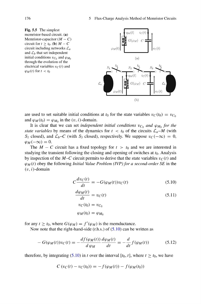
Fig. 5.5 The simplest
memristor-based circuit. (a)
Memristor-capacitor (M − C)
circuit for t ≥ t 0 . (b) M − C
circuit including networks L a
and L b that set independent
initial conditions v C 0 and ϕ M 0
through the evolution of the
electrical variables v C (t) and
ϕ M (t) for t < t 0
G(ϕ M ) C
i C (t)
q M (t)
v C (t)
ϕ M (t)
G(ϕ M ) C
(a)
(b)
L a
L b
S 1
t 0
S 2
t 0
S 3
t 0
i C (t)
q M (t)
v C (t)
ϕ M (t)
are used to set suitable initial conditions at t 0 for the state variables v C (t 0 ) = v C 0
and ϕ M (t 0 ) = ϕ M 0 in the (v, i)-domain.
It is clear that we can set independent initial conditions v C 0 and ϕ M 0 for the
state variables by means of the dynamics for t < t 0 of the circuits L a –M (with
S 1 closed), and L b –C (with S 3 closed), respectively. We suppose v C (−∞) = 0,
ϕ M (−∞) = 0.
The M − C circuit has a fixed topology for t > t 0 and we are interested in
studying the transient following the closing and opening of switches at t 0 . Analysis
by inspection of the M–C circuit permits to derive that the state variables v C (t) and
ϕ M (t) obey the following Initial Value Problem (IVP) for a second-order SE in the
(v, i)-domain
C
dv C (t)
dt
= −G(ϕ M (t))v C (t)
(5.10)
dϕ M (t)
dt
= v C (t)
(5.11)
v C (t 0 ) = v C 0
ϕ M (t 0 ) = ϕ M 0
for any t ≥ t 0 , where G(ϕ M ) = f (ϕ M ) is the memductance.
Now note that the right-hand-side (r.h.s.) of (5.10) can be written as
− G(ϕ M (t))v C (t) = −
df (ϕ M (t))
d ϕ M
dϕ M (t)
dt
= −
d
dt
f (ϕ M (t))
(5.12)
therefore, by integrating (5.10) in t over the interval [t 0 , t], where t ≥ t 0 , we have
C (v C (t) − v C (t 0 )) = −f (ϕ M (t)) − f (ϕ M (t 0 ))
5 Flux-Charge Analysis Method of Memristor Circuits
Fig. 5.5 The simplest
memristor-based circuit. (a)
Memristor-capacitor (M − C)
circuit for t ≥ t 0 . (b) M − C
circuit including networks L a
and L b that set independent
initial conditions v C 0 and ϕ M 0
through the evolution of the
electrical variables v C (t) and
ϕ M (t) for t < t 0
G(ϕ M ) C
i C (t)
q M (t)
v C (t)
ϕ M (t)
G(ϕ M ) C
(a)
(b)
L a
L b
S 1
t 0
S 2
t 0
S 3
t 0
i C (t)
q M (t)
v C (t)
ϕ M (t)
are used to set suitable initial conditions at t 0 for the state variables v C (t 0 ) = v C 0
and ϕ M (t 0 ) = ϕ M 0 in the (v, i)-domain.
It is clear that we can set independent initial conditions v C 0 and ϕ M 0 for the
state variables by means of the dynamics for t < t 0 of the circuits L a –M (with
S 1 closed), and L b –C (with S 3 closed), respectively. We suppose v C (−∞) = 0,
ϕ M (−∞) = 0.
The M − C circuit has a fixed topology for t > t 0 and we are interested in
studying the transient following the closing and opening of switches at t 0 . Analysis
by inspection of the M–C circuit permits to derive that the state variables v C (t) and
ϕ M (t) obey the following Initial Value Problem (IVP) for a second-order SE in the
(v, i)-domain
C
dv C (t)
dt
= −G(ϕ M (t))v C (t)
(5.10)
dϕ M (t)
dt
= v C (t)
(5.11)
v C (t 0 ) = v C 0
ϕ M (t 0 ) = ϕ M 0
for any t ≥ t 0 , where G(ϕ M ) = f (ϕ M ) is the memductance.
Now note that the right-hand-side (r.h.s.) of (5.10) can be written as
− G(ϕ M (t))v C (t) = −
df (ϕ M (t))
d ϕ M
dϕ M (t)
dt
= −
d
dt
f (ϕ M (t))
(5.12)
therefore, by integrating (5.10) in t over the interval [t 0 , t], where t ≥ t 0 , we have
C (v C (t) − v C (t 0 )) = −f (ϕ M (t)) − f (ϕ M (t 0 ))