

5.2 Forms of Kirchhoff Laws in the Flux-Charge Domain
167
that it gives answers that do not agree with measurements) when the velocity ν of
a body approaches the velocity of light c. Thanks to Einstein’s Special Theory of
Relativity [5], it can be shown that Newton’s Second Law must be replaced by its
relativistic version
f =
m 0 a
1 −
ν 2
c 2
3
(5.2)
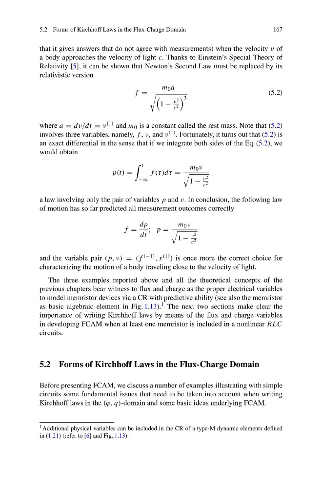
where a = dν/dt = ν (1) and m 0 is a constant called the rest mass. Note that (5.2)
involves three variables, namely, f , ν, and ν (1) . Fortunately, it turns out that (5.2) is
an exact differential in the sense that if we integrate both sides of the Eq. (5.2), we
would obtain
p(t) =
t
−∞
f (τ )dτ =
m 0 ν
1 −
ν 2
c 2
a law involving only the pair of variables p and ν. In conclusion, the following law
of motion has so far predicted all measurement outcomes correctly
f =
dp
dt
; p =
m 0 ν
1 −
ν 2
c 2
and the variable pair (p, ν) = (f (−1) , x (1) ) is once more the correct choice for
characterizing the motion of a body traveling close to the velocity of light.
The three examples reported above and all the theoretical concepts of the
previous chapters bear witness to flux and charge as the proper electrical variables
to model memristor devices via a CR with predictive ability (see also the memristor
as basic algebraic element in Fig. 1.13). 1 The next two sections make clear the
importance of writing Kirchhoff laws by means of the flux and charge variables
in developing FCAM when at least one memristor is included in a nonlinear RLC
circuits.
5.2 Forms of Kirchhoff Laws in the Flux-Charge Domain
Before presenting FCAM, we discuss a number of examples illustrating with simple
circuits some fundamental issues that need to be taken into account when writing
Kirchhoff laws in the (ϕ, q)-domain and some basic ideas underlying FCAM.
1 Additional physical variables can be included in the CR of a type-M dynamic elements defined
in (1.21) (refer to [6] and Fig. 1.13).
167
that it gives answers that do not agree with measurements) when the velocity ν of
a body approaches the velocity of light c. Thanks to Einstein’s Special Theory of
Relativity [5], it can be shown that Newton’s Second Law must be replaced by its
relativistic version
f =
m 0 a
1 −
ν 2
c 2
3
(5.2)
where a = dν/dt = ν (1) and m 0 is a constant called the rest mass. Note that (5.2)
involves three variables, namely, f , ν, and ν (1) . Fortunately, it turns out that (5.2) is
an exact differential in the sense that if we integrate both sides of the Eq. (5.2), we
would obtain
p(t) =
t
−∞
f (τ )dτ =
m 0 ν
1 −
ν 2
c 2
a law involving only the pair of variables p and ν. In conclusion, the following law
of motion has so far predicted all measurement outcomes correctly
f =
dp
dt
; p =
m 0 ν
1 −
ν 2
c 2
and the variable pair (p, ν) = (f (−1) , x (1) ) is once more the correct choice for
characterizing the motion of a body traveling close to the velocity of light.
The three examples reported above and all the theoretical concepts of the
previous chapters bear witness to flux and charge as the proper electrical variables
to model memristor devices via a CR with predictive ability (see also the memristor
as basic algebraic element in Fig. 1.13). 1 The next two sections make clear the
importance of writing Kirchhoff laws by means of the flux and charge variables
in developing FCAM when at least one memristor is included in a nonlinear RLC
circuits.
5.2 Forms of Kirchhoff Laws in the Flux-Charge Domain
Before presenting FCAM, we discuss a number of examples illustrating with simple
circuits some fundamental issues that need to be taken into account when writing
Kirchhoff laws in the (ϕ, q)-domain and some basic ideas underlying FCAM.
1 Additional physical variables can be included in the CR of a type-M dynamic elements defined
in (1.21) (refer to [6] and Fig. 1.13).