

or:
T e (r k (r, Q)χ( Q) + T N ( Q k (r, Q)χ ( Q)
+V e (r, Q k (r, Q)χ( Q) + V N ( Q) k (r, Q)χ ( Q)
= E
el
k · k (r, Q)χ( Q) + E
v
k− k (r, Q)χ ( Q)
(3.2.10)
Let us space the terms on the left and right sides of (3.2.10), which are functions
of r and Q into separate equations and reduce again wave functions on which
operators do not act:
b
T e ðrÞ þ b
V e ðr; QÞ
h
i
U k ðr; QÞ ¼ E
el
k Á U k ðr; QÞ
ð 3:2:11Þ
b
T N ðQÞ þ b
V N ðQÞ
h
i
vðQÞ ¼ E
v
k vðQÞ
ð 3:2:12Þ
Equation (3.2.11) is entirely identical to (3.2.3), and, there is E
el
k , not U k (Q) on
(3.2.11) rhs, only.
The physical meaning of the obtained results can be illustrated by the example of
the PEC of a diatomic molecule:
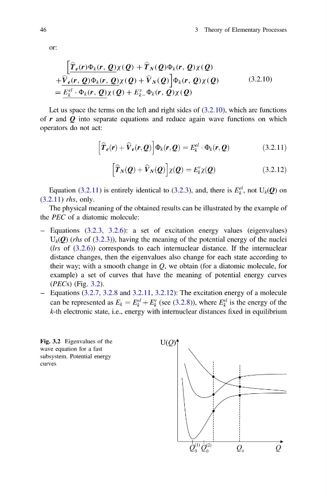
– Equations (3.2.3, 3.2.6): a set of excitation energy values (eigenvalues)
U k (Q) (rhs of (3.2.3)), having the meaning of the potential energy of the nuclei
(lrs of (3.2.6)) corresponds to each internuclear distance. If the internuclear
distance changes, then the eigenvalues also change for each state according to
their way; with a smooth change in Q, we obtain (for a diatomic molecule, for
example) a set of curves that have the meaning of potential energy curves
(PECs) (Fig. 3.2).
– Equations (3.2.7, 3.2.8 and 3.2.11, 3.2.12): The excitation energy of a molecule
can be represented as E k ¼ E
el
k þ E
v
k (see (3.2.8)), where E
el
k is the energy of the
k-th electronic state, i.e., energy with internuclear distances fixed in equilibrium
Fig. 3.2 Eigenvalues of the
wave equation for a fast
subsystem. Potential energy
curves
46
3 Theory of Elementary Processes
T e (r k (r, Q)χ( Q) + T N ( Q k (r, Q)χ ( Q)
+V e (r, Q k (r, Q)χ( Q) + V N ( Q) k (r, Q)χ ( Q)
= E
el
k · k (r, Q)χ( Q) + E
v
k− k (r, Q)χ ( Q)
(3.2.10)
Let us space the terms on the left and right sides of (3.2.10), which are functions
of r and Q into separate equations and reduce again wave functions on which
operators do not act:
b
T e ðrÞ þ b
V e ðr; QÞ
h
i
U k ðr; QÞ ¼ E
el
k Á U k ðr; QÞ
ð 3:2:11Þ
b
T N ðQÞ þ b
V N ðQÞ
h
i
vðQÞ ¼ E
v
k vðQÞ
ð 3:2:12Þ
Equation (3.2.11) is entirely identical to (3.2.3), and, there is E
el
k , not U k (Q) on
(3.2.11) rhs, only.
The physical meaning of the obtained results can be illustrated by the example of
the PEC of a diatomic molecule:
– Equations (3.2.3, 3.2.6): a set of excitation energy values (eigenvalues)
U k (Q) (rhs of (3.2.3)), having the meaning of the potential energy of the nuclei
(lrs of (3.2.6)) corresponds to each internuclear distance. If the internuclear
distance changes, then the eigenvalues also change for each state according to
their way; with a smooth change in Q, we obtain (for a diatomic molecule, for
example) a set of curves that have the meaning of potential energy curves
(PECs) (Fig. 3.2).
– Equations (3.2.7, 3.2.8 and 3.2.11, 3.2.12): The excitation energy of a molecule
can be represented as E k ¼ E
el
k þ E
v
k (see (3.2.8)), where E
el
k is the energy of the
k-th electronic state, i.e., energy with internuclear distances fixed in equilibrium
Fig. 3.2 Eigenvalues of the
wave equation for a fast
subsystem. Potential energy
curves
46
3 Theory of Elementary Processes