

~ T ¼ n 1 ~ a þ n 2 ~ b þ n 3 ~ c
ð1:3Þ
where n 1 , n 2 and n 3 are arbitrary integers, when putting together in the form [n 1
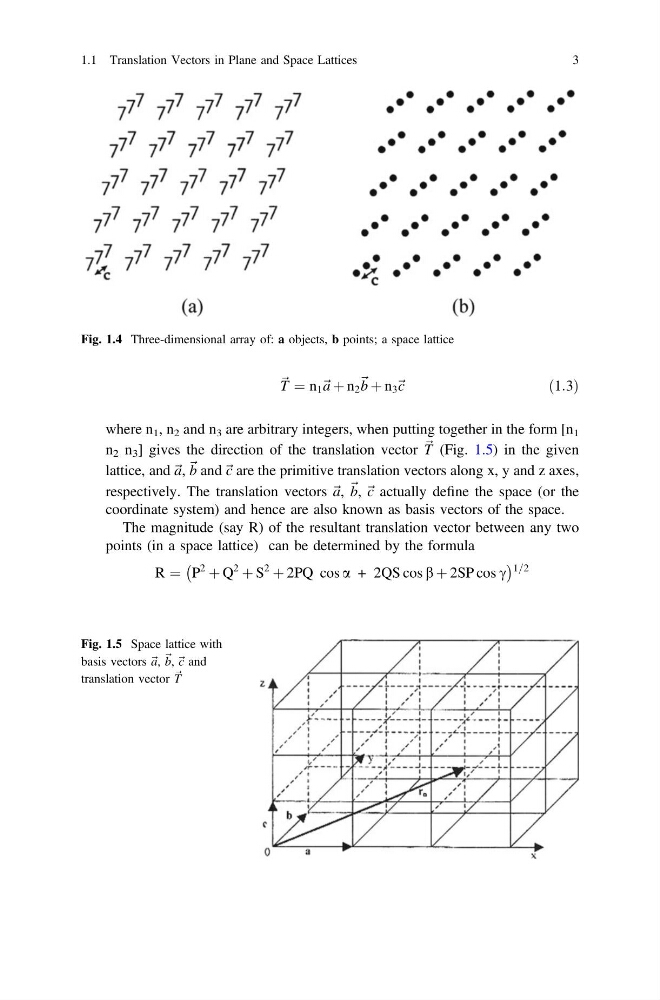
n 2 n 3 ] gives the direction of the translation vector ~ T (Fig. 1.5) in the given
lattice, and ~ a, ~ b and ~ c are the primitive translation vectors along x, y and z axes,
respectively. The translation vectors ~ a, ~ b, ~ c actually define the space (or the
coordinate system) and hence are also known as basis vectors of the space.
The magnitude (say R) of the resultant translation vector between any two
points (in a space lattice) can be determined by the formula
R ¼ P
2
þ Q
2
þ S
2
þ 2PQ cos a + 2QS cos b þ 2SP cos c
À
Á 1=2
Fig. 1.4 Three-dimensional array of: a objects, b points; a space lattice
Fig. 1.5 Space lattice with
basis vectors ~ a, ~ b, ~ c and
translation vector ~ T
1.1 Translation Vectors in Plane and Space Lattices
3
ð1:3Þ
where n 1 , n 2 and n 3 are arbitrary integers, when putting together in the form [n 1
n 2 n 3 ] gives the direction of the translation vector ~ T (Fig. 1.5) in the given
lattice, and ~ a, ~ b and ~ c are the primitive translation vectors along x, y and z axes,
respectively. The translation vectors ~ a, ~ b, ~ c actually define the space (or the
coordinate system) and hence are also known as basis vectors of the space.
The magnitude (say R) of the resultant translation vector between any two
points (in a space lattice) can be determined by the formula
R ¼ P
2
þ Q
2
þ S
2
þ 2PQ cos a + 2QS cos b þ 2SP cos c
À
Á 1=2
Fig. 1.4 Three-dimensional array of: a objects, b points; a space lattice
Fig. 1.5 Space lattice with
basis vectors ~ a, ~ b, ~ c and
translation vector ~ T
1.1 Translation Vectors in Plane and Space Lattices
3