

60
L. Rondoni
J t =
t
t 0
dt
R(t − t
)F(t
)
(1.215)
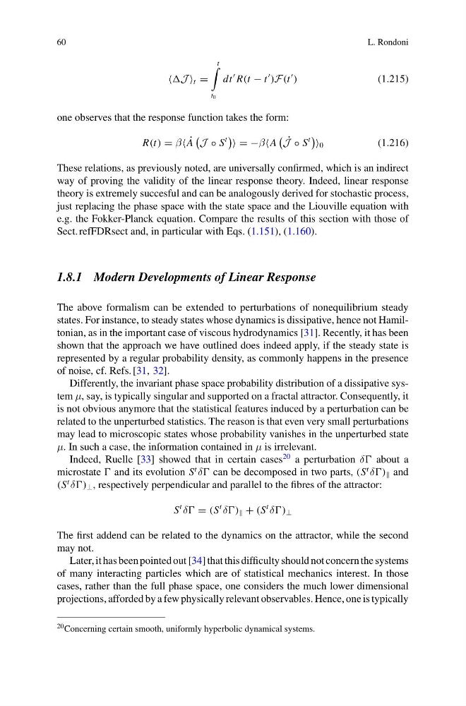
one observes that the response function takes the form:
R(t) = β ˙
A
J ◦ S
t
= −βA
˙
J ◦ S
t
0
(1.216)
These relations, as previously noted, are universally confirmed, which is an indirect
way of proving the validity of the linear response theory. Indeed, linear response
theory is extremely succesful and can be analogously derived for stochastic process,
just replacing the phase space with the state space and the Liouville equation with
e.g. the Fokker-Planck equation. Compare the results of this section with those of
Sect. refFDRsect and, in particular with Eqs. (1.151), (1.160).
1.8.1 Modern Developments of Linear Response
The above formalism can be extended to perturbations of nonequilibrium steady
states. For instance, to steady states whose dynamics is dissipative, hence not Hamiltonian, as in the important case of viscous hydrodynamics [31]. Recently, it has been
shown that the approach we have outlined does indeed apply, if the steady state is
represented by a regular probability density, as commonly happens in the presence
of noise, cf. Refs. [31, 32].
Differently, the invariant phase space probability distribution of a dissipative system μ, say, is typically singular and supported on a fractal attractor. Consequently, it
is not obvious anymore that the statistical features induced by a perturbation can be
related to the unperturbed statistics. The reason is that even very small perturbations
may lead to microscopic states whose probability vanishes in the unperturbed state
μ. In such a case, the information contained in μ is irrelevant.
Indeed, Ruelle [33] showed that in certain cases
20 a perturbation δ about a
microstate and its evolution S
t
δ can be decomposed in two parts, (S
t
δ) and
(S
t
δ) ⊥ , respectively perpendicular and parallel to the fibres of the attractor:
S
t
δ = (S
t
δ) + (S
t
δ) ⊥
The first addend can be related to the dynamics on the attractor, while the second
may not.
Later, it has been pointed out [34] that this difficulty should not concern the systems
of many interacting particles which are of statistical mechanics interest. In those
cases, rather than the full phase space, one considers the much lower dimensional
projections, afforded by a few physically relevant observables. Hence, one is typically
20 Concerning certain smooth, uniformly hyperbolic dynamical systems.
L. Rondoni
J t =
t
t 0
dt
R(t − t
)F(t
)
(1.215)
one observes that the response function takes the form:
R(t) = β ˙
A
J ◦ S
t
= −βA
˙
J ◦ S
t
0
(1.216)
These relations, as previously noted, are universally confirmed, which is an indirect
way of proving the validity of the linear response theory. Indeed, linear response
theory is extremely succesful and can be analogously derived for stochastic process,
just replacing the phase space with the state space and the Liouville equation with
e.g. the Fokker-Planck equation. Compare the results of this section with those of
Sect. refFDRsect and, in particular with Eqs. (1.151), (1.160).
1.8.1 Modern Developments of Linear Response
The above formalism can be extended to perturbations of nonequilibrium steady
states. For instance, to steady states whose dynamics is dissipative, hence not Hamiltonian, as in the important case of viscous hydrodynamics [31]. Recently, it has been
shown that the approach we have outlined does indeed apply, if the steady state is
represented by a regular probability density, as commonly happens in the presence
of noise, cf. Refs. [31, 32].
Differently, the invariant phase space probability distribution of a dissipative system μ, say, is typically singular and supported on a fractal attractor. Consequently, it
is not obvious anymore that the statistical features induced by a perturbation can be
related to the unperturbed statistics. The reason is that even very small perturbations
may lead to microscopic states whose probability vanishes in the unperturbed state
μ. In such a case, the information contained in μ is irrelevant.
Indeed, Ruelle [33] showed that in certain cases
20 a perturbation δ about a
microstate and its evolution S
t
δ can be decomposed in two parts, (S
t
δ) and
(S
t
δ) ⊥ , respectively perpendicular and parallel to the fibres of the attractor:
S
t
δ = (S
t
δ) + (S
t
δ) ⊥
The first addend can be related to the dynamics on the attractor, while the second
may not.
Later, it has been pointed out [34] that this difficulty should not concern the systems
of many interacting particles which are of statistical mechanics interest. In those
cases, rather than the full phase space, one considers the much lower dimensional
projections, afforded by a few physically relevant observables. Hence, one is typically
20 Concerning certain smooth, uniformly hyperbolic dynamical systems.