

26
L. Rondoni
P =
1
T
T
0
I (t)I
∗
(t)dt =
1
T
∞
n=−∞
∞
m=−∞
a n a
∗
m
T
0
e
i(ω n −ω m ) dT =
∞
n=−∞
|a n |
2
(1.85)
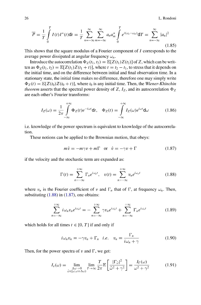
This shows that the square modulus of a Fourier component of I corresponds to the
average power dissipated at angular frequency ω n .
Introduce the autocorrelation Z (t 1 , t 2 ) = E[Z (t 1 )Z (t 2 )] of Z , which can be written as Z (t 1 , t 2 ) = E[Z (t 1 )Z (t 1 + t)], where t = t 2 − t 1 , to stress that it depends on
the initial time, and on the difference between initial and final observation time. In a
stationary state, the initial time makes no difference, therefore one may simply write
Z (t) = E[Z (t 0 )Z (t 0 + t)], where t 0 is any initial time. Then, the Wiener-Khinchin
theorem asserts that the spectral power density of Z , I Z , and its autocorrelation Z
are each other’s Fourier transforms:
I Z (ω) =
1
2π
+∞
−∞
Z (t)e
−iωt dt, , Z (t) =
+∞
−∞
I Z (ω)e
iωt dω
(1.86)
i.e. knowledge of the power spectrum is equivalent to knowledge of the autocorrelation.
These notions can be applied to the Brownian motion, that obeys:
m ˙
v = −mγv + m or ˙
v = −γv +
(1.87)
if the velocity and the stochastic term are expanded as:
(t) =
+∞
n=−∞
n e
iω n t
, v(t) =
+∞
n=−∞
v n e
iω n t
(1.88)
where v n is the Fourier coefficient of v and n that of , at frequency ω n . Then,
substituting (1.88) in (1.87), one obtains:
+∞
n=−∞
iω n v n e
iω n t
= −
+∞
n=−∞
γv n e
iω n t
+
+∞
n=−∞
n e
iω n t
(1.89)
which holds for all times t ∈ [0, T ] if and only if
iω n v n = −γv n + n i.e. v n =
n
iω n + γ
(1.90)
Then, for the power spectra of v and , we get:
I v (ω) =
lim
ω→0
ˆ
ω∈[ω,ω+ω)
lim
T →∞
T
2π
E
| ˆ
ω |
2
ˆ
ω 2 + γ 2
=
I (ω)
ω 2 + γ 2
(1.91)
L. Rondoni
P =
1
T
T
0
I (t)I
∗
(t)dt =
1
T
∞
n=−∞
∞
m=−∞
a n a
∗
m
T
0
e
i(ω n −ω m ) dT =
∞
n=−∞
|a n |
2
(1.85)
This shows that the square modulus of a Fourier component of I corresponds to the
average power dissipated at angular frequency ω n .
Introduce the autocorrelation Z (t 1 , t 2 ) = E[Z (t 1 )Z (t 2 )] of Z , which can be written as Z (t 1 , t 2 ) = E[Z (t 1 )Z (t 1 + t)], where t = t 2 − t 1 , to stress that it depends on
the initial time, and on the difference between initial and final observation time. In a
stationary state, the initial time makes no difference, therefore one may simply write
Z (t) = E[Z (t 0 )Z (t 0 + t)], where t 0 is any initial time. Then, the Wiener-Khinchin
theorem asserts that the spectral power density of Z , I Z , and its autocorrelation Z
are each other’s Fourier transforms:
I Z (ω) =
1
2π
+∞
−∞
Z (t)e
−iωt dt, , Z (t) =
+∞
−∞
I Z (ω)e
iωt dω
(1.86)
i.e. knowledge of the power spectrum is equivalent to knowledge of the autocorrelation.
These notions can be applied to the Brownian motion, that obeys:
m ˙
v = −mγv + m or ˙
v = −γv +
(1.87)
if the velocity and the stochastic term are expanded as:
(t) =
+∞
n=−∞
n e
iω n t
, v(t) =
+∞
n=−∞
v n e
iω n t
(1.88)
where v n is the Fourier coefficient of v and n that of , at frequency ω n . Then,
substituting (1.88) in (1.87), one obtains:
+∞
n=−∞
iω n v n e
iω n t
= −
+∞
n=−∞
γv n e
iω n t
+
+∞
n=−∞
n e
iω n t
(1.89)
which holds for all times t ∈ [0, T ] if and only if
iω n v n = −γv n + n i.e. v n =
n
iω n + γ
(1.90)
Then, for the power spectra of v and , we get:
I v (ω) =
lim
ω→0
ˆ
ω∈[ω,ω+ω)
lim
T →∞
T
2π
E
| ˆ
ω |
2
ˆ
ω 2 + γ 2
=
I (ω)
ω 2 + γ 2
(1.91)