

24
L. Rondoni
consider that we have a Gaussian process, hence the PDF’s of its variables observed
at different times are jointly Gaussian.
1.4 Fluctuation-Dissipation Theorem
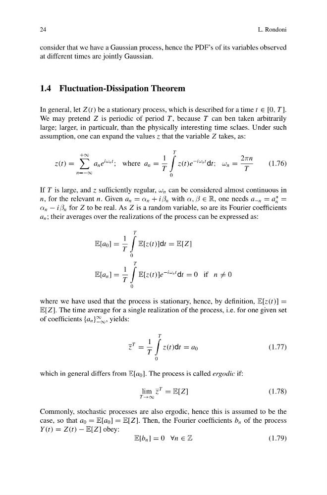
In general, let Z (t) be a stationary process, which is described for a time t ∈ [0, T ].
We may pretend Z is periodic of period T , because T can ben taken arbitrarily
large; larger, in particualr, than the physically interesting time sclaes. Under such
assumption, one can expand the values z that the variable Z takes, as:
z(t) =
+∞
n=−∞
a n e
iω n t
; where a n =
1
T
T
0
z(t)e
−iω n t dt; ω n =
2πn
T
(1.76)
If T is large, and z sufficiently regular, ω n can be considered almost continuous in
n, for the relevant n. Given a n = α n + iβ n with α, β ∈ R, one needs a −n = a
∗
n =
α n − iβ n for Z to be real. As Z is a random variable, so are its Fourier coefficients
a n ; their averages over the realizations of the process can be expressed as:
E[a 0 ] =
1
T
T
0
E[z(t)]dt = E[Z ]
E[a n ] =
1
T
T
0
E[z(t)]e
−iω n t dt = 0 if n = 0
where we have used that the process is stationary, hence, by definition, E[z(t)] =
E[Z ]. The time average for a single realization of the process, i.e. for one given set
of coefficients {a n }
∞
−∞ , yields:
z
T
=
1
T
T
0
z(t)dt = a 0
(1.77)
which in general differs from E[a 0 ]. The process is called ergodic if:
lim
T →∞
z
T
= E[Z ]
(1.78)
Commonly, stochastic processes are also ergodic, hence this is assumed to be the
case, so that a 0 = E[a 0 ] = E[Z ]. Then, the Fourier coefficients b n of the process
Y (t) = Z (t) − E[Z ] obey:
E[b n ] = 0 ∀n ∈ Z
(1.79)
L. Rondoni
consider that we have a Gaussian process, hence the PDF’s of its variables observed
at different times are jointly Gaussian.
1.4 Fluctuation-Dissipation Theorem
In general, let Z (t) be a stationary process, which is described for a time t ∈ [0, T ].
We may pretend Z is periodic of period T , because T can ben taken arbitrarily
large; larger, in particualr, than the physically interesting time sclaes. Under such
assumption, one can expand the values z that the variable Z takes, as:
z(t) =
+∞
n=−∞
a n e
iω n t
; where a n =
1
T
T
0
z(t)e
−iω n t dt; ω n =
2πn
T
(1.76)
If T is large, and z sufficiently regular, ω n can be considered almost continuous in
n, for the relevant n. Given a n = α n + iβ n with α, β ∈ R, one needs a −n = a
∗
n =
α n − iβ n for Z to be real. As Z is a random variable, so are its Fourier coefficients
a n ; their averages over the realizations of the process can be expressed as:
E[a 0 ] =
1
T
T
0
E[z(t)]dt = E[Z ]
E[a n ] =
1
T
T
0
E[z(t)]e
−iω n t dt = 0 if n = 0
where we have used that the process is stationary, hence, by definition, E[z(t)] =
E[Z ]. The time average for a single realization of the process, i.e. for one given set
of coefficients {a n }
∞
−∞ , yields:
z
T
=
1
T
T
0
z(t)dt = a 0
(1.77)
which in general differs from E[a 0 ]. The process is called ergodic if:
lim
T →∞
z
T
= E[Z ]
(1.78)
Commonly, stochastic processes are also ergodic, hence this is assumed to be the
case, so that a 0 = E[a 0 ] = E[Z ]. Then, the Fourier coefficients b n of the process
Y (t) = Z (t) − E[Z ] obey:
E[b n ] = 0 ∀n ∈ Z
(1.79)