

5 Basics of Molecular Modeling and Molecular Simulation
239
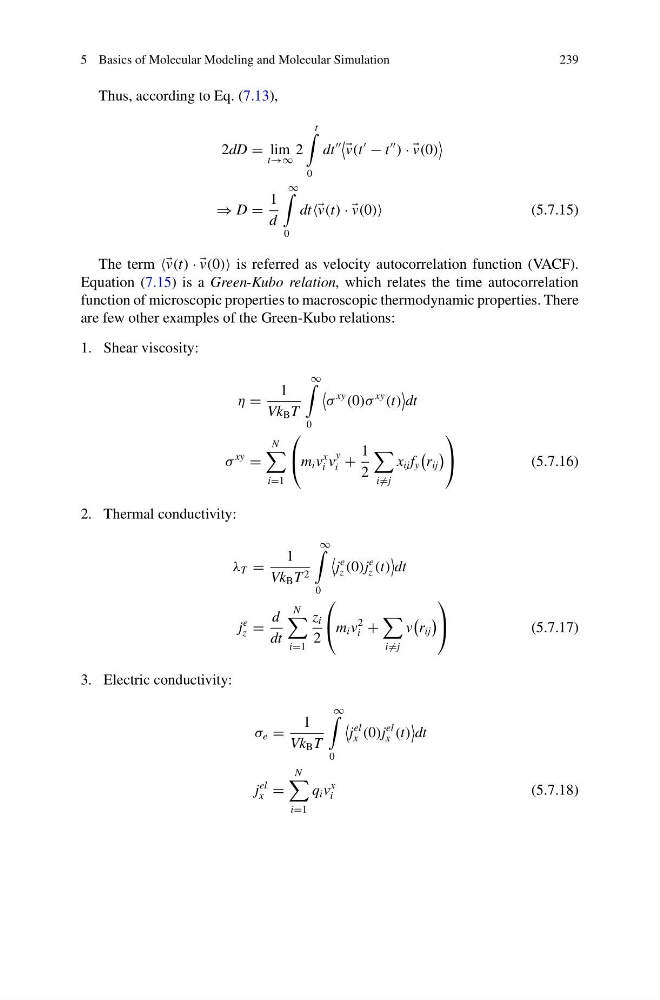
Thus, according to Eq. (7.13),
2dD = lim
t→∞
2
t
0
dt
v(t
− t
) · ·
v(0)
⇒ D =
1
d
∞
0
dt v(t) · ·
v(0)
(5.7.15)
The term v(t) · ·
v(0) is referred as velocity autocorrelation function (VACF).
Equation (7.15) is a Green-Kubo relation, which relates the time autocorrelation
function of microscopic properties to macroscopic thermodynamic properties. There
are few other examples of the Green-Kubo relations:
1. Shear viscosity:
η =
1
Vk B T
∞
0
σ
xy
(0)σ
xy
(t)
dt
σ
xy
=
N
i=1
⎛
⎝ m i v
x
i v
y
i +
1
2
i =j
x ij f y
r ij
⎞
⎠
(5.7.16)
2. Thermal conductivity:
λ T =
1
Vk B T 2
∞
0
j
e
z (0)j
e
z (t)
dt
j
e
z =
d
dt
N
i=1
z i
2
⎛
⎝ m i v
2
i +
i =j
v
r ij
⎞
⎠
(5.7.17)
3. Electric conductivity:
σ e =
1
Vk B T
∞
0
j
el
x (0)j
el
x (t)
dt
j
el
x =
N
i=1
q i v
x
i
(5.7.18)
239
Thus, according to Eq. (7.13),
2dD = lim
t→∞
2
t
0
dt
v(t
− t
) · ·
v(0)
⇒ D =
1
d
∞
0
dt v(t) · ·
v(0)
(5.7.15)
The term v(t) · ·
v(0) is referred as velocity autocorrelation function (VACF).
Equation (7.15) is a Green-Kubo relation, which relates the time autocorrelation
function of microscopic properties to macroscopic thermodynamic properties. There
are few other examples of the Green-Kubo relations:
1. Shear viscosity:
η =
1
Vk B T
∞
0
σ
xy
(0)σ
xy
(t)
dt
σ
xy
=
N
i=1
⎛
⎝ m i v
x
i v
y
i +
1
2
i =j
x ij f y
r ij
⎞
⎠
(5.7.16)
2. Thermal conductivity:
λ T =
1
Vk B T 2
∞
0
j
e
z (0)j
e
z (t)
dt
j
e
z =
d
dt
N
i=1
z i
2
⎛
⎝ m i v
2
i +
i =j
v
r ij
⎞
⎠
(5.7.17)
3. Electric conductivity:
σ e =
1
Vk B T
∞
0
j
el
x (0)j
el
x (t)
dt
j
el
x =
N
i=1
q i v
x
i
(5.7.18)