

5 Basics of Molecular Modeling and Molecular Simulation
229
⎧
⎪ ⎪ ⎪ ⎨
⎪ ⎪ ⎪ ⎩
x
predicted
0
(t + t) = x 0 (t) + x 1 (t) + x 2 (t) + x 3 (t)
x
predicted
1
(t + t) = x 1 (t) + 2x 2 (t) + 3x 3 (t)
x
predicted
2
(t + t) = x 2 (t) + 3x 3 (t)
x
predicted
3
(t + t) = x 3 (t)
(5.6.14)
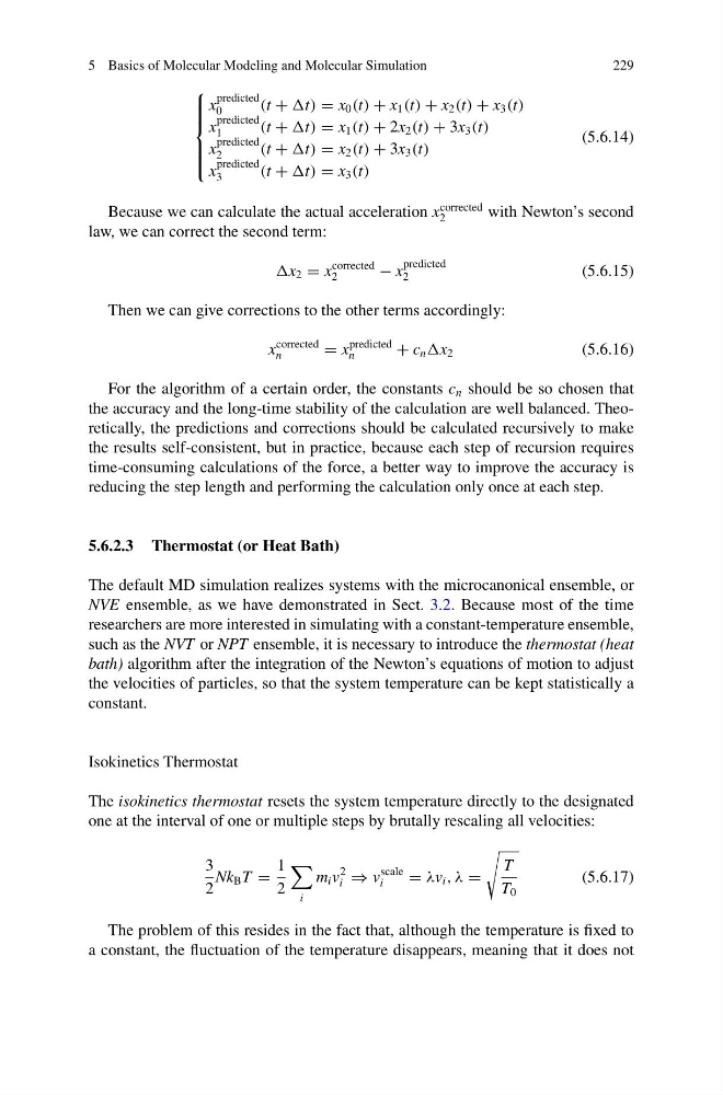
Because we can calculate the actual acceleration x
corrected
2
with Newton’s second
law, we can correct the second term:
x 2 = x
corrected
2
− x
predicted
2
(5.6.15)
Then we can give corrections to the other terms accordingly:
x
corrected
n
= x
predicted
n
+ c n x 2
(5.6.16)
For the algorithm of a certain order, the constants c n should be so chosen that
the accuracy and the long-time stability of the calculation are well balanced. Theoretically, the predictions and corrections should be calculated recursively to make
the results self-consistent, but in practice, because each step of recursion requires
time-consuming calculations of the force, a better way to improve the accuracy is
reducing the step length and performing the calculation only once at each step.
5.6.2.3 Thermostat (or Heat Bath)
The default MD simulation realizes systems with the microcanonical ensemble, or
NVE ensemble, as we have demonstrated in Sect. 3.2. Because most of the time
researchers are more interested in simulating with a constant-temperature ensemble,
such as the NVT or NPT ensemble, it is necessary to introduce the thermostat (heat
bath) algorithm after the integration of the Newton’s equations of motion to adjust
the velocities of particles, so that the system temperature can be kept statistically a
constant.
Isokinetics Thermostat
The isokinetics thermostat resets the system temperature directly to the designated
one at the interval of one or multiple steps by brutally rescaling all velocities:
3
2
Nk B T =
1
2
i
m i v
2
i ⇒ v
scale
i
= λv i , λ =
T
T 0
(5.6.17)
The problem of this resides in the fact that, although the temperature is fixed to
a constant, the fluctuation of the temperature disappears, meaning that it does not
229
⎧
⎪ ⎪ ⎪ ⎨
⎪ ⎪ ⎪ ⎩
x
predicted
0
(t + t) = x 0 (t) + x 1 (t) + x 2 (t) + x 3 (t)
x
predicted
1
(t + t) = x 1 (t) + 2x 2 (t) + 3x 3 (t)
x
predicted
2
(t + t) = x 2 (t) + 3x 3 (t)
x
predicted
3
(t + t) = x 3 (t)
(5.6.14)
Because we can calculate the actual acceleration x
corrected
2
with Newton’s second
law, we can correct the second term:
x 2 = x
corrected
2
− x
predicted
2
(5.6.15)
Then we can give corrections to the other terms accordingly:
x
corrected
n
= x
predicted
n
+ c n x 2
(5.6.16)
For the algorithm of a certain order, the constants c n should be so chosen that
the accuracy and the long-time stability of the calculation are well balanced. Theoretically, the predictions and corrections should be calculated recursively to make
the results self-consistent, but in practice, because each step of recursion requires
time-consuming calculations of the force, a better way to improve the accuracy is
reducing the step length and performing the calculation only once at each step.
5.6.2.3 Thermostat (or Heat Bath)
The default MD simulation realizes systems with the microcanonical ensemble, or
NVE ensemble, as we have demonstrated in Sect. 3.2. Because most of the time
researchers are more interested in simulating with a constant-temperature ensemble,
such as the NVT or NPT ensemble, it is necessary to introduce the thermostat (heat
bath) algorithm after the integration of the Newton’s equations of motion to adjust
the velocities of particles, so that the system temperature can be kept statistically a
constant.
Isokinetics Thermostat
The isokinetics thermostat resets the system temperature directly to the designated
one at the interval of one or multiple steps by brutally rescaling all velocities:
3
2
Nk B T =
1
2
i
m i v
2
i ⇒ v
scale
i
= λv i , λ =
T
T 0
(5.6.17)
The problem of this resides in the fact that, although the temperature is fixed to
a constant, the fluctuation of the temperature disappears, meaning that it does not