

14
L. Rondoni
+
t1
0
dt
1
t2
0
dt
2 e
−γ(t1+t2−t
1 −t
2 ) E[(t
1 ))(t
2 )]
= v
2
0 e
−γ(t1+t2) +
t1
0
dt
1
t2
0
dt
2 e
−γ(t1+t2−t
1 −t
2 ) qδ(t
1 − t
2 )
(1.25)
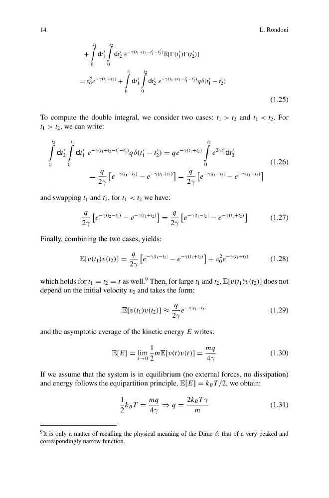
To compute the double integral, we consider two cases: t 1 > t 2 and t 1 < t 2 . For
t 1 > t 2 , we can write:
t 2
0
dt
2
t 1
0
dt
1 e
−γ(t 1 +t 2 −t
1 −t
2 ) qδ(t
1 − t
2 ) = qe
−γ(t 1 +t 2 )
t 2
0
e
2γt
2 dt
2
=
q
2γ
e
−γ(t 1 −t 2 )
− e
−γ(t 1 +t 2 )
=
q
2γ
e
−γ|t 1 −t 2 |
− e
−γ(t 1 +t 2 )
(1.26)
and swapping t 1 and t 2 , for t 1 < t 2 we have:
q
2γ
e
−γ(t 2 −t 1 )
− e
−γ(t 1 +t 2 )
=
q
2γ
e
−γ|t 1 −t 2 |
− e
−γ(t 1 +t 2 )
(1.27)
Finally, combining the two cases, yields:
E[v(t 1 )v(t 2 )] =
q
2γ
e
−γ|t 1 −t 2 |
− e
−γ(t 1 +t 2 )
+ v
2
0 e
−γ(t 1 +t 2 )
(1.28)
which holds for t 1 = t 2 = t as well.
9 Then, for large t 1 and t 2 , E[v(t 1 )v(t 2 )] does not
depend on the initial velocity v 0 and takes the form:
E[v(t 1 )v(t 2 )] ≈
q
2γ
e
−γ|t 1 −t 2 |
(1.29)
and the asymptotic average of the kinetic energy E writes:
E[E] = lim
t→0
1
2
mE[v(t)v(t)] =
mq
4γ
(1.30)
If we assume that the system is in equilibrium (no external forces, no dissipation)
and energy follows the equipartition principle, E[E] = k B T /2, we obtain:
1
2
k B T =
mq
4γ
⇒ q =
2k B T γ
m
(1.31)
9 It is only a matter of recalling the physical meaning of the Dirac δ: that of a very peaked and
correspondingly narrow function.
L. Rondoni
+
t1
0
dt
1
t2
0
dt
2 e
−γ(t1+t2−t
1 −t
2 ) E[(t
1 ))(t
2 )]
= v
2
0 e
−γ(t1+t2) +
t1
0
dt
1
t2
0
dt
2 e
−γ(t1+t2−t
1 −t
2 ) qδ(t
1 − t
2 )
(1.25)
To compute the double integral, we consider two cases: t 1 > t 2 and t 1 < t 2 . For
t 1 > t 2 , we can write:
t 2
0
dt
2
t 1
0
dt
1 e
−γ(t 1 +t 2 −t
1 −t
2 ) qδ(t
1 − t
2 ) = qe
−γ(t 1 +t 2 )
t 2
0
e
2γt
2 dt
2
=
q
2γ
e
−γ(t 1 −t 2 )
− e
−γ(t 1 +t 2 )
=
q
2γ
e
−γ|t 1 −t 2 |
− e
−γ(t 1 +t 2 )
(1.26)
and swapping t 1 and t 2 , for t 1 < t 2 we have:
q
2γ
e
−γ(t 2 −t 1 )
− e
−γ(t 1 +t 2 )
=
q
2γ
e
−γ|t 1 −t 2 |
− e
−γ(t 1 +t 2 )
(1.27)
Finally, combining the two cases, yields:
E[v(t 1 )v(t 2 )] =
q
2γ
e
−γ|t 1 −t 2 |
− e
−γ(t 1 +t 2 )
+ v
2
0 e
−γ(t 1 +t 2 )
(1.28)
which holds for t 1 = t 2 = t as well.
9 Then, for large t 1 and t 2 , E[v(t 1 )v(t 2 )] does not
depend on the initial velocity v 0 and takes the form:
E[v(t 1 )v(t 2 )] ≈
q
2γ
e
−γ|t 1 −t 2 |
(1.29)
and the asymptotic average of the kinetic energy E writes:
E[E] = lim
t→0
1
2
mE[v(t)v(t)] =
mq
4γ
(1.30)
If we assume that the system is in equilibrium (no external forces, no dissipation)
and energy follows the equipartition principle, E[E] = k B T /2, we obtain:
1
2
k B T =
mq
4γ
⇒ q =
2k B T γ
m
(1.31)
9 It is only a matter of recalling the physical meaning of the Dirac δ: that of a very peaked and
correspondingly narrow function.