

4 An Introduction to Emergence Dynamics in Complex Systems
189
ϕ j (t) = ϕ(t), j = 1, 2, . . . , N ,
(4.146)
i.e. all leaf oscillators are synchronous to each other while they are asynchronous
to the hub oscillator. The stability of this limit cycle can be analyzed in terms
of Floquet theory.
(2) Neutral State:
Type-II periodic solution occurs at some certain values of phase shifts. Let us
take the case α = 0 as an example, where Eqs. (4.140) can be simplified as
˙
x = K(
1
2
+ N )y
2
−
K
2
x
2
− ωy +
K
2
˙
y = −K(N + 1)xy + ωx
(4.147)
These two equations keep invariant under the time-reversal transformation.
R : (t, x, y) → (−t, −x, y).
(4.148)
This leads to an attracting set in the phase plane x > 0 and a repulsing set in the
phase plane x < 0. If an orbit passes the boundary x = 0 in both directions, this orbit
will be a closed type and neutrally stable. Therefore when α = 0 Eqs. (4.145) have
the neutral periodic solution, and this system is called a quasi-Hamiltonian system.
The corresponding collective state is called the neutral state (NS). The NS depends
on initial states, while the IPS is independent of initial states.
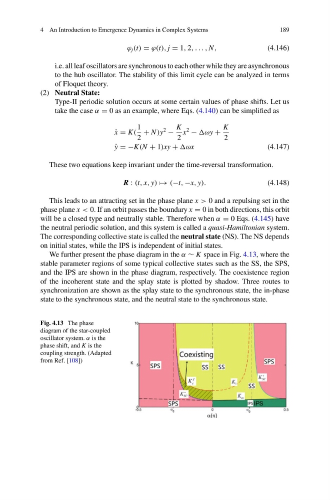
We further present the phase diagram in the α ∼ K space in Fig. 4.13, where the
stable parameter regions of some typical collective states such as the SS, the SPS,
and the IPS are shown in the phase diagram, respectively. The coexistence region
of the incoherent state and the splay state is plotted by shadow. Three routes to
synchronization are shown as the splay state to the synchronous state, the in-phase
state to the synchronous state, and the neutral state to the synchronous state.
Fig. 4.13 The phase
diagram of the star-coupled
oscillator system. α is the
phase shift, and K is the
coupling strength. (Adapted
from Ref. [108])
189
ϕ j (t) = ϕ(t), j = 1, 2, . . . , N ,
(4.146)
i.e. all leaf oscillators are synchronous to each other while they are asynchronous
to the hub oscillator. The stability of this limit cycle can be analyzed in terms
of Floquet theory.
(2) Neutral State:
Type-II periodic solution occurs at some certain values of phase shifts. Let us
take the case α = 0 as an example, where Eqs. (4.140) can be simplified as
˙
x = K(
1
2
+ N )y
2
−
K
2
x
2
− ωy +
K
2
˙
y = −K(N + 1)xy + ωx
(4.147)
These two equations keep invariant under the time-reversal transformation.
R : (t, x, y) → (−t, −x, y).
(4.148)
This leads to an attracting set in the phase plane x > 0 and a repulsing set in the
phase plane x < 0. If an orbit passes the boundary x = 0 in both directions, this orbit
will be a closed type and neutrally stable. Therefore when α = 0 Eqs. (4.145) have
the neutral periodic solution, and this system is called a quasi-Hamiltonian system.
The corresponding collective state is called the neutral state (NS). The NS depends
on initial states, while the IPS is independent of initial states.
We further present the phase diagram in the α ∼ K space in Fig. 4.13, where the
stable parameter regions of some typical collective states such as the SS, the SPS,
and the IPS are shown in the phase diagram, respectively. The coexistence region
of the incoherent state and the splay state is plotted by shadow. Three routes to
synchronization are shown as the splay state to the synchronous state, the in-phase
state to the synchronous state, and the neutral state to the synchronous state.
Fig. 4.13 The phase
diagram of the star-coupled
oscillator system. α is the
phase shift, and K is the
coupling strength. (Adapted
from Ref. [108])