

178
Z. Zheng
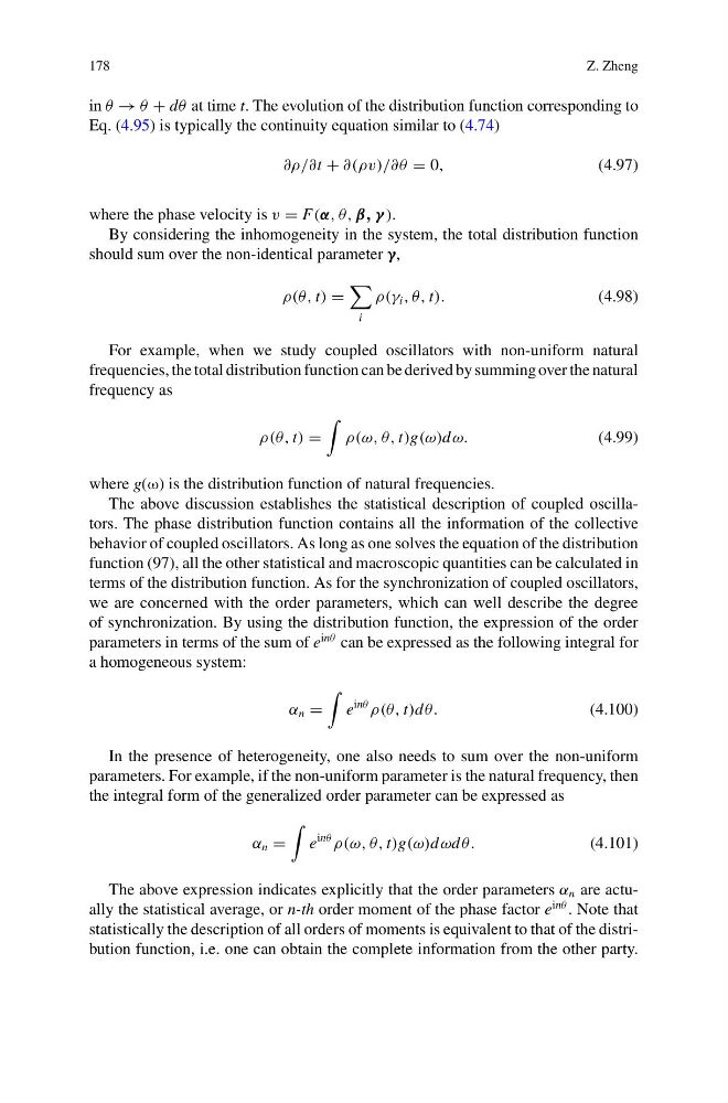
in θ → θ + dθ at time t. The evolution of the distribution function corresponding to
Eq. (4.95) is typically the continuity equation similar to (4.74)
∂ρ/∂t + ∂(ρv)/∂θ = 0,
(4.97)
where the phase velocity is v = F(α, θ, β, γ ).
By considering the inhomogeneity in the system, the total distribution function
should sum over the non-identical parameter γ,
ρ(θ, t) =
i
ρ(γ i , θ, t).
(4.98)
For example, when we study coupled oscillators with non-uniform natural
frequencies, the total distribution function can be derived by summing over the natural
frequency as
ρ(θ, t) =
ρ(ω, θ, t)g(ω)d ω.
(4.99)
where g(ω) is the distribution function of natural frequencies.
The above discussion establishes the statistical description of coupled oscillators. The phase distribution function contains all the information of the collective
behavior of coupled oscillators. As long as one solves the equation of the distribution
function (97), all the other statistical and macroscopic quantities can be calculated in
terms of the distribution function. As for the synchronization of coupled oscillators,
we are concerned with the order parameters, which can well describe the degree
of synchronization. By using the distribution function, the expression of the order
parameters in terms of the sum of e
inθ can be expressed as the following integral for
a homogeneous system:
α n =
e
inθ
ρ(θ, t)d θ.
(4.100)
In the presence of heterogeneity, one also needs to sum over the non-uniform
parameters. For example, if the non-uniform parameter is the natural frequency, then
the integral form of the generalized order parameter can be expressed as
α n =
e
inθ
ρ(ω, θ, t)g(ω)d ωd θ.
(4.101)
The above expression indicates explicitly that the order parameters α n are actually the statistical average, or n-th order moment of the phase factor e
inθ . Note that
statistically the description of all orders of moments is equivalent to that of the distribution function, i.e. one can obtain the complete information from the other party.
Z. Zheng
in θ → θ + dθ at time t. The evolution of the distribution function corresponding to
Eq. (4.95) is typically the continuity equation similar to (4.74)
∂ρ/∂t + ∂(ρv)/∂θ = 0,
(4.97)
where the phase velocity is v = F(α, θ, β, γ ).
By considering the inhomogeneity in the system, the total distribution function
should sum over the non-identical parameter γ,
ρ(θ, t) =
i
ρ(γ i , θ, t).
(4.98)
For example, when we study coupled oscillators with non-uniform natural
frequencies, the total distribution function can be derived by summing over the natural
frequency as
ρ(θ, t) =
ρ(ω, θ, t)g(ω)d ω.
(4.99)
where g(ω) is the distribution function of natural frequencies.
The above discussion establishes the statistical description of coupled oscillators. The phase distribution function contains all the information of the collective
behavior of coupled oscillators. As long as one solves the equation of the distribution
function (97), all the other statistical and macroscopic quantities can be calculated in
terms of the distribution function. As for the synchronization of coupled oscillators,
we are concerned with the order parameters, which can well describe the degree
of synchronization. By using the distribution function, the expression of the order
parameters in terms of the sum of e
inθ can be expressed as the following integral for
a homogeneous system:
α n =
e
inθ
ρ(θ, t)d θ.
(4.100)
In the presence of heterogeneity, one also needs to sum over the non-uniform
parameters. For example, if the non-uniform parameter is the natural frequency, then
the integral form of the generalized order parameter can be expressed as
α n =
e
inθ
ρ(ω, θ, t)g(ω)d ωd θ.
(4.101)
The above expression indicates explicitly that the order parameters α n are actually the statistical average, or n-th order moment of the phase factor e
inθ . Note that
statistically the description of all orders of moments is equivalent to that of the distribution function, i.e. one can obtain the complete information from the other party.