

128
Q. Wang
where
A 0 = 2ηδ αk δ βl + ( ¯
η −
2
3
η)δ γ k δ γ l δ αβ + α 1 (Q αk δ βl + δ αk Q βl )
+α 2 Q kl Q αβ + α 3 ( p α p k δ βl + δ αk p β p l ) + α 4 p k p l p α p β , A = ( p α δ βk + p β δ αk ). (3.133)
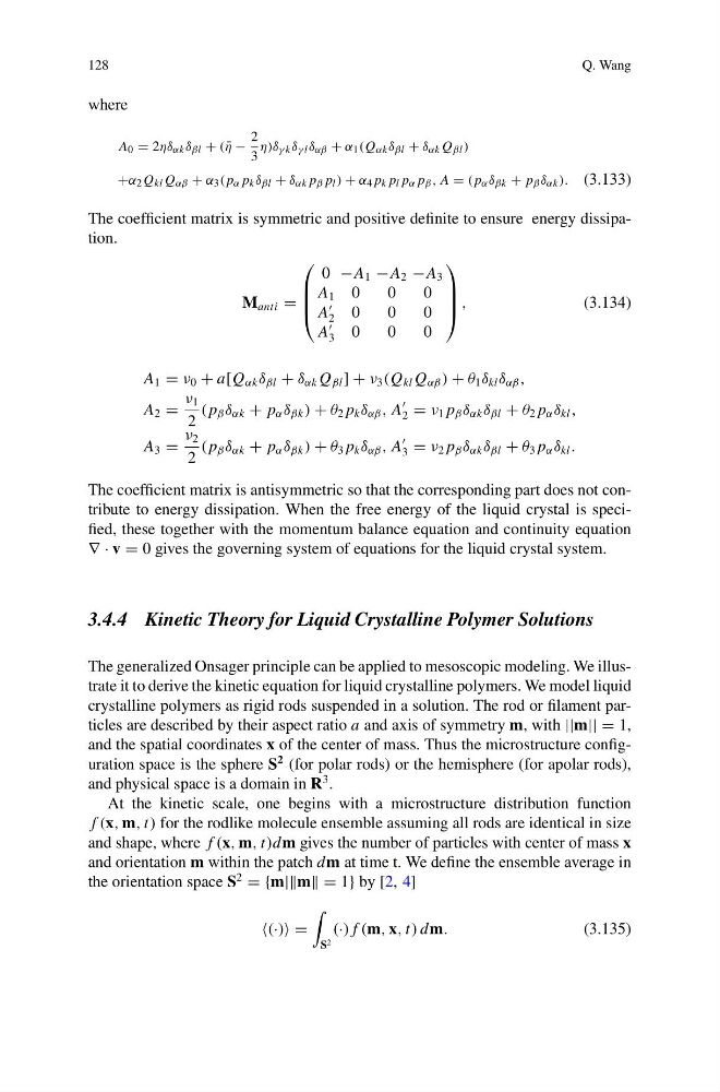
The coefficient matrix is symmetric and positive definite to ensure energy dissipation.
M anti =
⎛
⎜
⎜
⎝
0 −A 1 −A 2 −A 3
A 1 0
0
0
A
2
0
0
0
A
3
0
0
0
⎞
⎟
⎟
⎠ ,
(3.134)
A 1 = ν 0 + a[Q αk δ βl + δ αk Q βl ] + ν 3 (Q kl Q αβ ) + θ 1 δ kl δ αβ ,
A 2 =
ν 1
2
( p β δ αk + p α δ βk ) + θ 2 p k δ αβ , A
2 = ν 1 p β δ αk δ βl + θ 2 p α δ kl ,
A 3 =
ν 2
2
( p β δ αk + p α δ βk ) + θ 3 p k δ αβ , A
3 = ν 2 p β δ αk δ βl + θ 3 p α δ kl .
The coefficient matrix is antisymmetric so that the corresponding part does not contribute to energy dissipation. When the free energy of the liquid crystal is specified, these together with the momentum balance equation and continuity equation
∇ · v = 0 gives the governing system of equations for the liquid crystal system.
3.4.4 Kinetic Theory for Liquid Crystalline Polymer Solutions
The generalized Onsager principle can be applied to mesoscopic modeling. We illustrate it to derive the kinetic equation for liquid crystalline polymers. We model liquid
crystalline polymers as rigid rods suspended in a solution. The rod or filament particles are described by their aspect ratio a and axis of symmetry m, with ||m|| = 1,
and the spatial coordinates x of the center of mass. Thus the microstructure configuration space is the sphere S
2 (for polar rods) or the hemisphere (for apolar rods),
and physical space is a domain in R
3 .
At the kinetic scale, one begins with a microstructure distribution function
f (x, m, t) for the rodlike molecule ensemble assuming all rods are identical in size
and shape, where f (x, m, t)dm gives the number of particles with center of mass x
and orientation m within the patch dm at time t. We define the ensemble average in
the orientation space S
2
= {m||m = 1} by [2, 4]
(·) =
S 2
(·) f (m, x, t) dm.
(3.135)
Q. Wang
where
A 0 = 2ηδ αk δ βl + ( ¯
η −
2
3
η)δ γ k δ γ l δ αβ + α 1 (Q αk δ βl + δ αk Q βl )
+α 2 Q kl Q αβ + α 3 ( p α p k δ βl + δ αk p β p l ) + α 4 p k p l p α p β , A = ( p α δ βk + p β δ αk ). (3.133)
The coefficient matrix is symmetric and positive definite to ensure energy dissipation.
M anti =
⎛
⎜
⎜
⎝
0 −A 1 −A 2 −A 3
A 1 0
0
0
A
2
0
0
0
A
3
0
0
0
⎞
⎟
⎟
⎠ ,
(3.134)
A 1 = ν 0 + a[Q αk δ βl + δ αk Q βl ] + ν 3 (Q kl Q αβ ) + θ 1 δ kl δ αβ ,
A 2 =
ν 1
2
( p β δ αk + p α δ βk ) + θ 2 p k δ αβ , A
2 = ν 1 p β δ αk δ βl + θ 2 p α δ kl ,
A 3 =
ν 2
2
( p β δ αk + p α δ βk ) + θ 3 p k δ αβ , A
3 = ν 2 p β δ αk δ βl + θ 3 p α δ kl .
The coefficient matrix is antisymmetric so that the corresponding part does not contribute to energy dissipation. When the free energy of the liquid crystal is specified, these together with the momentum balance equation and continuity equation
∇ · v = 0 gives the governing system of equations for the liquid crystal system.
3.4.4 Kinetic Theory for Liquid Crystalline Polymer Solutions
The generalized Onsager principle can be applied to mesoscopic modeling. We illustrate it to derive the kinetic equation for liquid crystalline polymers. We model liquid
crystalline polymers as rigid rods suspended in a solution. The rod or filament particles are described by their aspect ratio a and axis of symmetry m, with ||m|| = 1,
and the spatial coordinates x of the center of mass. Thus the microstructure configuration space is the sphere S
2 (for polar rods) or the hemisphere (for apolar rods),
and physical space is a domain in R
3 .
At the kinetic scale, one begins with a microstructure distribution function
f (x, m, t) for the rodlike molecule ensemble assuming all rods are identical in size
and shape, where f (x, m, t)dm gives the number of particles with center of mass x
and orientation m within the patch dm at time t. We define the ensemble average in
the orientation space S
2
= {m||m = 1} by [2, 4]
(·) =
S 2
(·) f (m, x, t) dm.
(3.135)