

3 Generalized Onsager Principle and It Applications
103
where H is the negative Hessian matrix of the entropy function, which is a symmetric
and positive definite matrix (H > 0) at the maximum when S
has the
continuous second order derivatives. In fact, we can introduce a change of variables
near the equilibrium so that the entropy function is exactly a quadratic form of a
new set of thermodynamic variables x
in a neighborhood of the maximum. So,
without loss of generality, we assume the entropy function is a quadratic function of
thermodynamical variable x near the equilibrium. We note that this is plausible so
long as we are interested in the near equilibrium behavior of the thermodynamical
system. The probability density of thermodynamical variable x near the equilibrium
(when they are viewed as random fluctuations/variables) is related to via
f (x) =
1
Z
ex p[ B T ], where k B is the Boltzmann constant, T the absolute
temperature and Z is the partition function.
When the system deviates from equilibrium, spontaneous irreversible processes
arise in response to the generalized thermodynamic force X conjugate to x defined
by
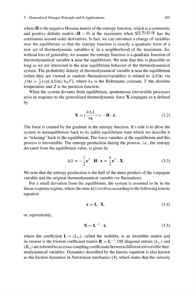
X = (
∂∂S
∂x
) = −H · x.
(3.2)
The force is created by the gradient in the entropy function. It’s role is to drive the
system in nonequilibrium back to its stable equilibrium state which we describe it
as “relaxing” back to the equilibrium. The force vanishes at the equilibrium and this
process is irreversible. The entropy production during the process, i.e., the entropy
deviated from the equilibrium value, is given by
= −
1
2
x
T
· H · x =
1
2
x
T
· X.
(3.3)
We note that the entropy production is the half of the inner product of the conjugate
variable and the original thermodynamical variable (or fluctuation).
For a small deviation from the equilibrium, the system is assumed to be in the
linear response regime, where the state x(t) evolves according to the following kinetic
equation
˙
x = L · X,
(3.4)
or, equivalently,
X = L
−1
· ˙
x,
(3.5)
where the coefficient L = (L i j ), called the mobility, is an invertible matrix and
its inverse is the friction coefficient matrix R = L
−1 . Off-diagonal entries (L i j ) and
(R i j ) are referred to as cross-coupling coefficients between different irreversible thermodynamical variables. Dynamics described by the kinetic equation is also known
as the friction dynamics in Newtonian mechanics [4], which states that the velocity
103
where H is the negative Hessian matrix of the entropy function, which is a symmetric
and positive definite matrix (H > 0) at the maximum when S
has the
continuous second order derivatives. In fact, we can introduce a change of variables
near the equilibrium so that the entropy function is exactly a quadratic form of a
new set of thermodynamic variables x
in a neighborhood of the maximum. So,
without loss of generality, we assume the entropy function is a quadratic function of
thermodynamical variable x near the equilibrium. We note that this is plausible so
long as we are interested in the near equilibrium behavior of the thermodynamical
system. The probability density of thermodynamical variable x near the equilibrium
(when they are viewed as random fluctuations/variables) is related to via
f (x) =
1
Z
ex p[ B T ], where k B is the Boltzmann constant, T the absolute
temperature and Z is the partition function.
When the system deviates from equilibrium, spontaneous irreversible processes
arise in response to the generalized thermodynamic force X conjugate to x defined
by
X = (
∂∂S
∂x
) = −H · x.
(3.2)
The force is created by the gradient in the entropy function. It’s role is to drive the
system in nonequilibrium back to its stable equilibrium state which we describe it
as “relaxing” back to the equilibrium. The force vanishes at the equilibrium and this
process is irreversible. The entropy production during the process, i.e., the entropy
deviated from the equilibrium value, is given by
= −
1
2
x
T
· H · x =
1
2
x
T
· X.
(3.3)
We note that the entropy production is the half of the inner product of the conjugate
variable and the original thermodynamical variable (or fluctuation).
For a small deviation from the equilibrium, the system is assumed to be in the
linear response regime, where the state x(t) evolves according to the following kinetic
equation
˙
x = L · X,
(3.4)
or, equivalently,
X = L
−1
· ˙
x,
(3.5)
where the coefficient L = (L i j ), called the mobility, is an invertible matrix and
its inverse is the friction coefficient matrix R = L
−1 . Off-diagonal entries (L i j ) and
(R i j ) are referred to as cross-coupling coefficients between different irreversible thermodynamical variables. Dynamics described by the kinetic equation is also known
as the friction dynamics in Newtonian mechanics [4], which states that the velocity