

5.4 Going Further: From Linear Stability Analysis to Oscillation Regimes
247
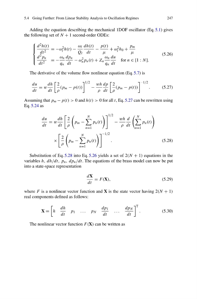
Adding the equation describing the mechanical 1DOF oscillator (Eq. 5.1) gives
the following set of N + 1 second-order ODEs:
⎧
⎪ ⎪ ⎨
⎪ ⎪ ⎩
d 2 h(t)
dt 2 = −ω 2
l h(t) −
ω l
Q l
dh(t)
dt
−
p(t)
μ
+ ω 2
l h 0 +
p m
μ
d 2 p n
dt 2 = −
ω n
q n
dp n
dt
− ω 2
n p n (t) + Z n
ω n
q n
du
dt
for n ∈ [1 : N ].
(5.26)
The derivative of the volume flow nonlinear equation (Eq. 5.7) is
du
dt
= w
dh
dt
2
ρ
(p m − p(t))
1/2
−
wh
ρ
dp
dt
2
ρ
(p m − p(t))
−1/2
.
(5.27)
Assuming that p m − p(t) > 0 and h(t) > 0 for all t, Eq. 5.27 can be rewritten using
Eq. 5.24 as
du
dt
= w
dh
dt
2
ρ
p m −
N
n=1
p n (t)
1/2
−
wh
ρ
d
dt
N
n=1
p n (t)
×
2
ρ
p m −
N
n=1
p n (t)
−1/2
.
(5.28)
Substitution of Eq. 5.28 into Eq. 5.26 yields a set of 2(N + 1) equations in the
variables h, dh/dt, p n , dp n /dt. The equations of the brass model can now be put
into a state-space representation
dX
dt
= F (X),
(5.29)
where F is a nonlinear vector function and X is the state vector having 2(N + 1)
real components defined as follows:
X =
h
dh
dt
p 1 . . . p N
dp 1
dt
. . .
dp N
dt
T
.
(5.30)
The nonlinear vector function F (X) can be written as
247
Adding the equation describing the mechanical 1DOF oscillator (Eq. 5.1) gives
the following set of N + 1 second-order ODEs:
⎧
⎪ ⎪ ⎨
⎪ ⎪ ⎩
d 2 h(t)
dt 2 = −ω 2
l h(t) −
ω l
Q l
dh(t)
dt
−
p(t)
μ
+ ω 2
l h 0 +
p m
μ
d 2 p n
dt 2 = −
ω n
q n
dp n
dt
− ω 2
n p n (t) + Z n
ω n
q n
du
dt
for n ∈ [1 : N ].
(5.26)
The derivative of the volume flow nonlinear equation (Eq. 5.7) is
du
dt
= w
dh
dt
2
ρ
(p m − p(t))
1/2
−
wh
ρ
dp
dt
2
ρ
(p m − p(t))
−1/2
.
(5.27)
Assuming that p m − p(t) > 0 and h(t) > 0 for all t, Eq. 5.27 can be rewritten using
Eq. 5.24 as
du
dt
= w
dh
dt
2
ρ
p m −
N
n=1
p n (t)
1/2
−
wh
ρ
d
dt
N
n=1
p n (t)
×
2
ρ
p m −
N
n=1
p n (t)
−1/2
.
(5.28)
Substitution of Eq. 5.28 into Eq. 5.26 yields a set of 2(N + 1) equations in the
variables h, dh/dt, p n , dp n /dt. The equations of the brass model can now be put
into a state-space representation
dX
dt
= F (X),
(5.29)
where F is a nonlinear vector function and X is the state vector having 2(N + 1)
real components defined as follows:
X =
h
dh
dt
p 1 . . . p N
dp 1
dt
. . .
dp N
dt
T
.
(5.30)
The nonlinear vector function F (X) can be written as