

5.3 Beyond Pianissimo: Modelling Realistic Playing Amplitudes
239
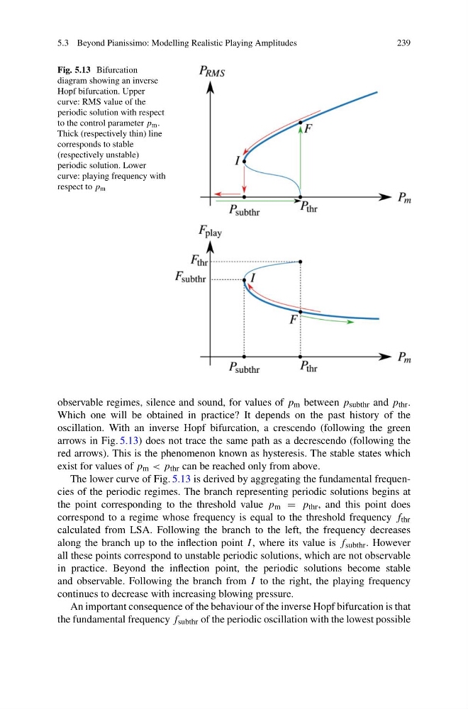
Fig. 5.13 Bifurcation
diagram showing an inverse
Hopf bifurcation. Upper
curve: RMS value of the
periodic solution with respect
to the control parameter p m .
Thick (respectively thin) line
corresponds to stable
(respectively unstable)
periodic solution. Lower
curve: playing frequency with
respect to p m
observable regimes, silence and sound, for values of p m between p subthr and p thr .
Which one will be obtained in practice? It depends on the past history of the
oscillation. With an inverse Hopf bifurcation, a crescendo (following the green
arrows in Fig. 5.13) does not trace the same path as a decrescendo (following the
red arrows). This is the phenomenon known as hysteresis. The stable states which
exist for values of p m < p thr can be reached only from above.
The lower curve of Fig. 5.13 is derived by aggregating the fundamental frequencies of the periodic regimes. The branch representing periodic solutions begins at
the point corresponding to the threshold value p m = p thr , and this point does
correspond to a regime whose frequency is equal to the threshold frequency f thr
calculated from LSA. Following the branch to the left, the frequency decreases
along the branch up to the inflection point I , where its value is f subthr . However
all these points correspond to unstable periodic solutions, which are not observable
in practice. Beyond the inflection point, the periodic solutions become stable
and observable. Following the branch from I to the right, the playing frequency
continues to decrease with increasing blowing pressure.
An important consequence of the behaviour of the inverse Hopf bifurcation is that
the fundamental frequency f subthr of the periodic oscillation with the lowest possible
239
Fig. 5.13 Bifurcation
diagram showing an inverse
Hopf bifurcation. Upper
curve: RMS value of the
periodic solution with respect
to the control parameter p m .
Thick (respectively thin) line
corresponds to stable
(respectively unstable)
periodic solution. Lower
curve: playing frequency with
respect to p m
observable regimes, silence and sound, for values of p m between p subthr and p thr .
Which one will be obtained in practice? It depends on the past history of the
oscillation. With an inverse Hopf bifurcation, a crescendo (following the green
arrows in Fig. 5.13) does not trace the same path as a decrescendo (following the
red arrows). This is the phenomenon known as hysteresis. The stable states which
exist for values of p m < p thr can be reached only from above.
The lower curve of Fig. 5.13 is derived by aggregating the fundamental frequencies of the periodic regimes. The branch representing periodic solutions begins at
the point corresponding to the threshold value p m = p thr , and this point does
correspond to a regime whose frequency is equal to the threshold frequency f thr
calculated from LSA. Following the branch to the left, the frequency decreases
along the branch up to the inflection point I , where its value is f subthr . However
all these points correspond to unstable periodic solutions, which are not observable
in practice. Beyond the inflection point, the periodic solutions become stable
and observable. Following the branch from I to the right, the playing frequency
continues to decrease with increasing blowing pressure.
An important consequence of the behaviour of the inverse Hopf bifurcation is that
the fundamental frequency f subthr of the periodic oscillation with the lowest possible