

202
4 After the Lips: Acoustic Resonances and Radiation
= cos(kL)
Ae
−jkx 2 + Be
jkx 2
+ j sin(kL)
Ae
−jkx 2 − Be
jkx 2
.
(4.92)
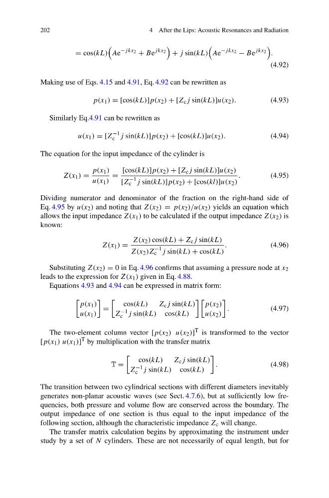
Making use of Eqs. 4.15 and 4.91, Eq. 4.92 can be rewritten as
p(x 1 ) = [cos(kL)]p(x 2 ) + [Z c j sin(kL)]u(x 2 ).
(4.93)
Similarly Eq.4.91 can be rewritten as
u(x 1 ) = [Z
−1
c j sin(kL)]p(x 2 ) + [cos(kL)]u(x 2 ).
(4.94)
The equation for the input impedance of the cylinder is
Z(x 1 ) =
p(x 1 )
u(x 1 )
=
[cos(kL)]p(x 2 ) + [Z c j sin(kL)]u(x 2 )
[Z
−1
c j sin(kL)]p(x 2 ) + [cos(kl)]u(x 2 )
.
(4.95)
Dividing numerator and denominator of the fraction on the right-hand side of
Eq. 4.95 by u(x 2 ) and noting that Z(x 2 ) = p(x 2 )/u(x 2 ) yields an equation which
allows the input impedance Z(x 1 ) to be calculated if the output impedance Z(x 2 ) is
known:
Z(x 1 ) =
Z(x 2 ) cos(kL) + Z c j sin(kL)
Z(x 2 )Z
−1
c j sin(kL) + cos(kL)
.
(4.96)
Substituting Z(x 2 ) = 0 in Eq. 4.96 confirms that assuming a pressure node at x 2
leads to the expression for Z(x 1 ) given in Eq. 4.88.
Equations 4.93 and 4.94 can be expressed in matrix form:
p(x 1 )
u(x 1 )
=
cos(kL) Z c j sin(kL)
Z −1
c j sin(kL) cos(kL)
p(x 2 )
u(x 2 )
.
(4.97)
The two-element column vector [p(x 2 ) u(x 2 )] T is transformed to the vector
[p(x 1 ) u(x 1 )] T by multiplication with the transfer matrix
T =
cos(kL) Z c j sin(kL)
Z −1
c j sin(kL) cos(kL)
.
(4.98)
The transition between two cylindrical sections with different diameters inevitably
generates non-planar acoustic waves (see Sect. 4.7.6), but at sufficiently low frequencies, both pressure and volume flow are conserved across the boundary. The
output impedance of one section is thus equal to the input impedance of the
following section, although the characteristic impedance Z c will change.
The transfer matrix calculation begins by approximating the instrument under
study by a set of N cylinders. These are not necessarily of equal length, but for
4 After the Lips: Acoustic Resonances and Radiation
= cos(kL)
Ae
−jkx 2 + Be
jkx 2
+ j sin(kL)
Ae
−jkx 2 − Be
jkx 2
.
(4.92)
Making use of Eqs. 4.15 and 4.91, Eq. 4.92 can be rewritten as
p(x 1 ) = [cos(kL)]p(x 2 ) + [Z c j sin(kL)]u(x 2 ).
(4.93)
Similarly Eq.4.91 can be rewritten as
u(x 1 ) = [Z
−1
c j sin(kL)]p(x 2 ) + [cos(kL)]u(x 2 ).
(4.94)
The equation for the input impedance of the cylinder is
Z(x 1 ) =
p(x 1 )
u(x 1 )
=
[cos(kL)]p(x 2 ) + [Z c j sin(kL)]u(x 2 )
[Z
−1
c j sin(kL)]p(x 2 ) + [cos(kl)]u(x 2 )
.
(4.95)
Dividing numerator and denominator of the fraction on the right-hand side of
Eq. 4.95 by u(x 2 ) and noting that Z(x 2 ) = p(x 2 )/u(x 2 ) yields an equation which
allows the input impedance Z(x 1 ) to be calculated if the output impedance Z(x 2 ) is
known:
Z(x 1 ) =
Z(x 2 ) cos(kL) + Z c j sin(kL)
Z(x 2 )Z
−1
c j sin(kL) + cos(kL)
.
(4.96)
Substituting Z(x 2 ) = 0 in Eq. 4.96 confirms that assuming a pressure node at x 2
leads to the expression for Z(x 1 ) given in Eq. 4.88.
Equations 4.93 and 4.94 can be expressed in matrix form:
p(x 1 )
u(x 1 )
=
cos(kL) Z c j sin(kL)
Z −1
c j sin(kL) cos(kL)
p(x 2 )
u(x 2 )
.
(4.97)
The two-element column vector [p(x 2 ) u(x 2 )] T is transformed to the vector
[p(x 1 ) u(x 1 )] T by multiplication with the transfer matrix
T =
cos(kL) Z c j sin(kL)
Z −1
c j sin(kL) cos(kL)
.
(4.98)
The transition between two cylindrical sections with different diameters inevitably
generates non-planar acoustic waves (see Sect. 4.7.6), but at sufficiently low frequencies, both pressure and volume flow are conserved across the boundary. The
output impedance of one section is thus equal to the input impedance of the
following section, although the characteristic impedance Z c will change.
The transfer matrix calculation begins by approximating the instrument under
study by a set of N cylinders. These are not necessarily of equal length, but for