

4.1 Internal Sounds in Brass Instruments
119
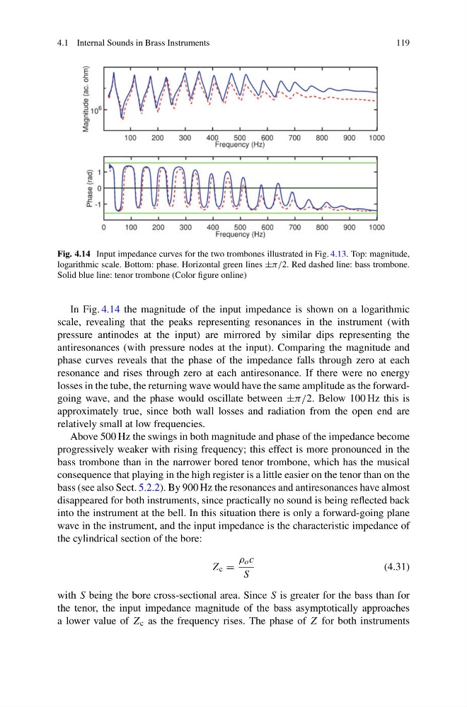
Fig. 4.14 Input impedance curves for the two trombones illustrated in Fig. 4.13. Top: magnitude,
logarithmic scale. Bottom: phase. Horizontal green lines ±π/2. Red dashed line: bass trombone.
Solid blue line: tenor trombone (Color figure online)
In Fig. 4.14 the magnitude of the input impedance is shown on a logarithmic
scale, revealing that the peaks representing resonances in the instrument (with
pressure antinodes at the input) are mirrored by similar dips representing the
antiresonances (with pressure nodes at the input). Comparing the magnitude and
phase curves reveals that the phase of the impedance falls through zero at each
resonance and rises through zero at each antiresonance. If there were no energy
losses in the tube, the returning wave would have the same amplitude as the forwardgoing wave, and the phase would oscillate between ±π/2. Below 100 Hz this is
approximately true, since both wall losses and radiation from the open end are
relatively small at low frequencies.
Above 500 Hz the swings in both magnitude and phase of the impedance become
progressively weaker with rising frequency; this effect is more pronounced in the
bass trombone than in the narrower bored tenor trombone, which has the musical
consequence that playing in the high register is a little easier on the tenor than on the
bass (see also Sect. 5.2.2). By 900 Hz the resonances and antiresonances have almost
disappeared for both instruments, since practically no sound is being reflected back
into the instrument at the bell. In this situation there is only a forward-going plane
wave in the instrument, and the input impedance is the characteristic impedance of
the cylindrical section of the bore:
Z c =
ρ o c
S
(4.31)
with S being the bore cross-sectional area. Since S is greater for the bass than for
the tenor, the input impedance magnitude of the bass asymptotically approaches
a lower value of Z c as the frequency rises. The phase of Z for both instruments
119
Fig. 4.14 Input impedance curves for the two trombones illustrated in Fig. 4.13. Top: magnitude,
logarithmic scale. Bottom: phase. Horizontal green lines ±π/2. Red dashed line: bass trombone.
Solid blue line: tenor trombone (Color figure online)
In Fig. 4.14 the magnitude of the input impedance is shown on a logarithmic
scale, revealing that the peaks representing resonances in the instrument (with
pressure antinodes at the input) are mirrored by similar dips representing the
antiresonances (with pressure nodes at the input). Comparing the magnitude and
phase curves reveals that the phase of the impedance falls through zero at each
resonance and rises through zero at each antiresonance. If there were no energy
losses in the tube, the returning wave would have the same amplitude as the forwardgoing wave, and the phase would oscillate between ±π/2. Below 100 Hz this is
approximately true, since both wall losses and radiation from the open end are
relatively small at low frequencies.
Above 500 Hz the swings in both magnitude and phase of the impedance become
progressively weaker with rising frequency; this effect is more pronounced in the
bass trombone than in the narrower bored tenor trombone, which has the musical
consequence that playing in the high register is a little easier on the tenor than on the
bass (see also Sect. 5.2.2). By 900 Hz the resonances and antiresonances have almost
disappeared for both instruments, since practically no sound is being reflected back
into the instrument at the bell. In this situation there is only a forward-going plane
wave in the instrument, and the input impedance is the characteristic impedance of
the cylindrical section of the bore:
Z c =
ρ o c
S
(4.31)
with S being the bore cross-sectional area. Since S is greater for the bass than for
the tenor, the input impedance magnitude of the bass asymptotically approaches
a lower value of Z c as the frequency rises. The phase of Z for both instruments