

5.2 Boltzmann Equation and Relic Density
75
χ h
2
0.12
x d
23
√
g ∗
10
1.7 × 10
−9 GeV
−2
σ χχ→ f f v
2.5 × 10
−10 GeV
−2
σ χχ→ f f v
,
(5.15)
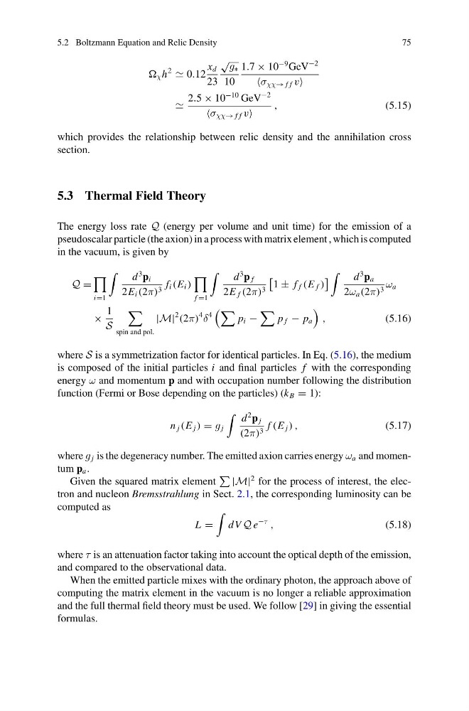
which provides the relationship between relic density and the annihilation cross
section.
5.3 Thermal Field Theory
The energy loss rate Q (energy per volume and unit time) for the emission of a
pseudoscalar particle (the axion) in a process with matrix element , which is computed
in the vacuum, is given by
Q =
i=1
d
3 p i
2E i (2π) 3 f i (E i )
f =1
d
3 p f
2E f (2π) 3
1 ± f f (E f )
d
3 p a
2ω a (2π) 3 ω a
×
1
S
spin and pol.
|M|
2
(2π)
4
δ
4
p i −
p f − p a
,
(5.16)
where S is a symmetrization factor for identical particles. In Eq. (5.16), the medium
is composed of the initial particles i and final particles f with the corresponding
energy ω and momentum p and with occupation number following the distribution
function (Fermi or Bose depending on the particles) (k B = 1):
n j (E j ) = g j
d
2 p j
(2π) 3 f (E j ) ,
(5.17)
where g j is the degeneracy number. The emitted axion carries energy ω a and momentum p a .
Given the squared matrix element
|M|
2 for the process of interest, the electron and nucleon Bremsstrahlung in Sect. 2.1, the corresponding luminosity can be
computed as
L =
dV Q e
−τ
,
(5.18)
where τ is an attenuation factor taking into account the optical depth of the emission,
and compared to the observational data.
When the emitted particle mixes with the ordinary photon, the approach above of
computing the matrix element in the vacuum is no longer a reliable approximation
and the full thermal field theory must be used. We follow [29] in giving the essential
formulas.
75
χ h
2
0.12
x d
23
√
g ∗
10
1.7 × 10
−9 GeV
−2
σ χχ→ f f v
2.5 × 10
−10 GeV
−2
σ χχ→ f f v
,
(5.15)
which provides the relationship between relic density and the annihilation cross
section.
5.3 Thermal Field Theory
The energy loss rate Q (energy per volume and unit time) for the emission of a
pseudoscalar particle (the axion) in a process with matrix element , which is computed
in the vacuum, is given by
Q =
i=1
d
3 p i
2E i (2π) 3 f i (E i )
f =1
d
3 p f
2E f (2π) 3
1 ± f f (E f )
d
3 p a
2ω a (2π) 3 ω a
×
1
S
spin and pol.
|M|
2
(2π)
4
δ
4
p i −
p f − p a
,
(5.16)
where S is a symmetrization factor for identical particles. In Eq. (5.16), the medium
is composed of the initial particles i and final particles f with the corresponding
energy ω and momentum p and with occupation number following the distribution
function (Fermi or Bose depending on the particles) (k B = 1):
n j (E j ) = g j
d
2 p j
(2π) 3 f (E j ) ,
(5.17)
where g j is the degeneracy number. The emitted axion carries energy ω a and momentum p a .
Given the squared matrix element
|M|
2 for the process of interest, the electron and nucleon Bremsstrahlung in Sect. 2.1, the corresponding luminosity can be
computed as
L =
dV Q e
−τ
,
(5.18)
where τ is an attenuation factor taking into account the optical depth of the emission,
and compared to the observational data.
When the emitted particle mixes with the ordinary photon, the approach above of
computing the matrix element in the vacuum is no longer a reliable approximation
and the full thermal field theory must be used. We follow [29] in giving the essential
formulas.