

236
Y. Dai and C. S. Tan
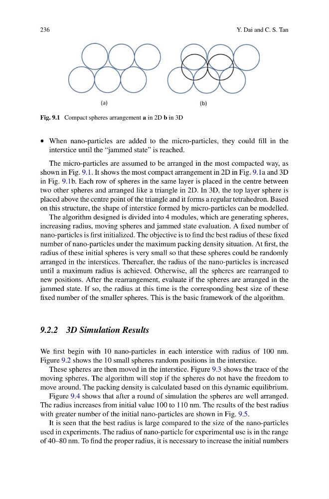
Fig. 9.1 Compact spheres arrangement a in 2D b in 3D
• When nano-particles are added to the micro-particles, they could fill in the
interstice until the “jammed state” is reached.
The micro-particles are assumed to be arranged in the most compacted way, as
shown in Fig. 9.1. It shows the most compact arrangement in 2D in Fig. 9.1a and 3D
in Fig. 9.1b. Each row of spheres in the same layer is placed in the centre between
two other spheres and arranged like a triangle in 2D. In 3D, the top layer sphere is
placed above the centre point of the triangle and it forms a regular tetrahedron. Based
on this structure, the shape of interstice formed by micro-particles can be modelled.
The algorithm designed is divided into 4 modules, which are generating spheres,
increasing radius, moving spheres and jammed state evaluation. A fixed number of
nano-particles is first initialized. The objective is to find the best radius of these fixed
number of nano-particles under the maximum packing density situation. At first, the
radius of these initial spheres is very small so that these spheres could be randomly
arranged in the interstices. Thereafter, the radius of the nano-particles is increased
until a maximum radius is achieved. Otherwise, all the spheres are rearranged to
new positions. After the rearrangement, evaluate if the spheres are arranged in the
jammed state. If so, the radius at this time is the corresponding best size of these
fixed number of the smaller spheres. This is the basic framework of the algorithm.
9.2.2 3D Simulation Results
We first begin with 10 nano-particles in each interstice with radius of 100 nm.
Figure 9.2 shows the 10 small spheres random positions in the interstice.
These spheres are then moved in the interstice. Figure 9.3 shows the trace of the
moving spheres. The algorithm will stop if the spheres do not have the freedom to
move around. The packing density is calculated based on this dynamic equilibrium.
Figure 9.4 shows that after a round of simulation the spheres are well arranged.
The radius increases from initial value 100 to 110 nm. The results of the best radius
with greater number of the initial nano-particles are shown in Fig. 9.5.
It is seen that the best radius is large compared to the size of the nano-particles
used in experiments. The radius of nano-particle for experimental use is in the range
of 40–80 nm. To find the proper radius, it is necessary to increase the initial numbers
Y. Dai and C. S. Tan
Fig. 9.1 Compact spheres arrangement a in 2D b in 3D
• When nano-particles are added to the micro-particles, they could fill in the
interstice until the “jammed state” is reached.
The micro-particles are assumed to be arranged in the most compacted way, as
shown in Fig. 9.1. It shows the most compact arrangement in 2D in Fig. 9.1a and 3D
in Fig. 9.1b. Each row of spheres in the same layer is placed in the centre between
two other spheres and arranged like a triangle in 2D. In 3D, the top layer sphere is
placed above the centre point of the triangle and it forms a regular tetrahedron. Based
on this structure, the shape of interstice formed by micro-particles can be modelled.
The algorithm designed is divided into 4 modules, which are generating spheres,
increasing radius, moving spheres and jammed state evaluation. A fixed number of
nano-particles is first initialized. The objective is to find the best radius of these fixed
number of nano-particles under the maximum packing density situation. At first, the
radius of these initial spheres is very small so that these spheres could be randomly
arranged in the interstices. Thereafter, the radius of the nano-particles is increased
until a maximum radius is achieved. Otherwise, all the spheres are rearranged to
new positions. After the rearrangement, evaluate if the spheres are arranged in the
jammed state. If so, the radius at this time is the corresponding best size of these
fixed number of the smaller spheres. This is the basic framework of the algorithm.
9.2.2 3D Simulation Results
We first begin with 10 nano-particles in each interstice with radius of 100 nm.
Figure 9.2 shows the 10 small spheres random positions in the interstice.
These spheres are then moved in the interstice. Figure 9.3 shows the trace of the
moving spheres. The algorithm will stop if the spheres do not have the freedom to
move around. The packing density is calculated based on this dynamic equilibrium.
Figure 9.4 shows that after a round of simulation the spheres are well arranged.
The radius increases from initial value 100 to 110 nm. The results of the best radius
with greater number of the initial nano-particles are shown in Fig. 9.5.
It is seen that the best radius is large compared to the size of the nano-particles
used in experiments. The radius of nano-particle for experimental use is in the range
of 40–80 nm. To find the proper radius, it is necessary to increase the initial numbers