

5 Phase-Field-Crystal Model: A Tool for Probing Atoms in TSV
119
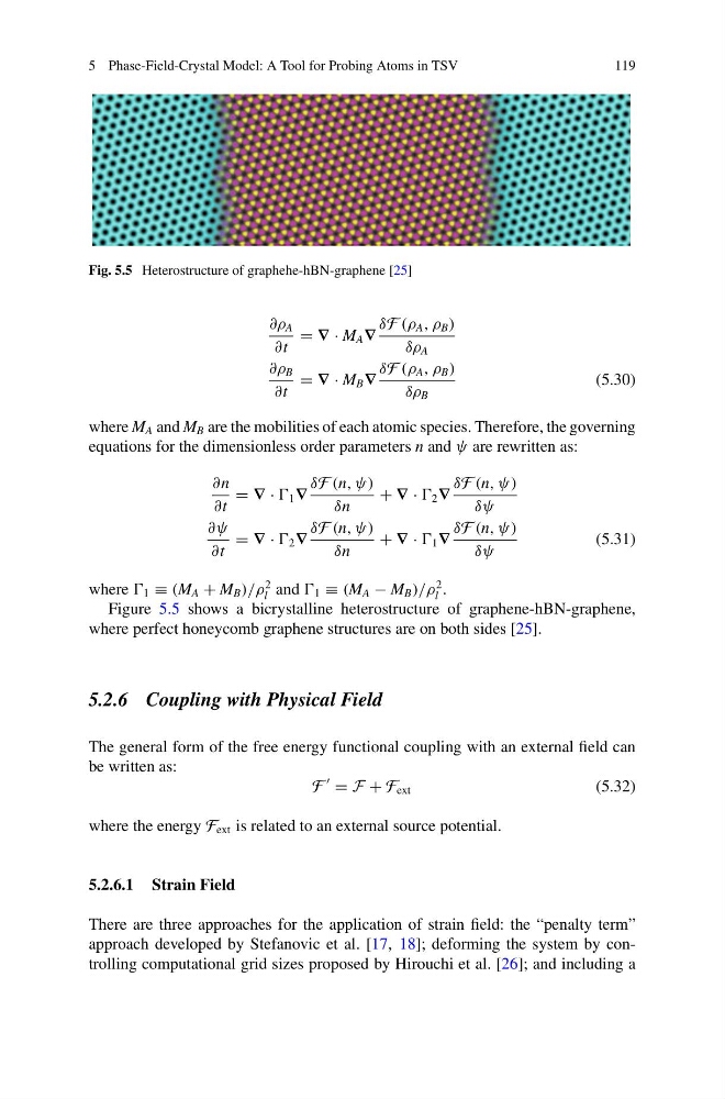
Fig. 5.5 Heterostructure of graphehe-hBN-graphene [25]
∂ρ A
∂t
= ∇ · M A ∇
δF (ρ A , ρ B )
δρ A
∂ρ B
∂t
= ∇ · M B ∇
δF (ρ A , ρ B )
δρ B
(5.30)
where M A and M B are the mobilities of each atomic species. Therefore, the governing
equations for the dimensionless order parameters n and ψ are rewritten as:
∂n
∂t
= ∇ · 1 ∇
δF (n, ψ)
δn
+ ∇ · 2 ∇
δF (n, ψ)
δψ
∂ψ
∂t
= ∇ · 2 ∇
δF (n, ψ)
δn
+ ∇ · 1 ∇
δF (n, ψ)
δψ
(5.31)
where 1 ≡ (M A + M B )/ρ
2
l and 1 ≡ (M A − M B )/ρ
2
l .
Figure 5.5 shows a bicrystalline heterostructure of graphene-hBN-graphene,
where perfect honeycomb graphene structures are on both sides [25].
5.2.6 Coupling with Physical Field
The general form of the free energy functional coupling with an external field can
be written as:
F
= F + F ext
(5.32)
where the energy F ext is related to an external source potential.
5.2.6.1 Strain Field
There are three approaches for the application of strain field: the “penalty term”
approach developed by Stefanovic et al. [17, 18]; deforming the system by controlling computational grid sizes proposed by Hirouchi et al. [26]; and including a
119
Fig. 5.5 Heterostructure of graphehe-hBN-graphene [25]
∂ρ A
∂t
= ∇ · M A ∇
δF (ρ A , ρ B )
δρ A
∂ρ B
∂t
= ∇ · M B ∇
δF (ρ A , ρ B )
δρ B
(5.30)
where M A and M B are the mobilities of each atomic species. Therefore, the governing
equations for the dimensionless order parameters n and ψ are rewritten as:
∂n
∂t
= ∇ · 1 ∇
δF (n, ψ)
δn
+ ∇ · 2 ∇
δF (n, ψ)
δψ
∂ψ
∂t
= ∇ · 2 ∇
δF (n, ψ)
δn
+ ∇ · 1 ∇
δF (n, ψ)
δψ
(5.31)
where 1 ≡ (M A + M B )/ρ
2
l and 1 ≡ (M A − M B )/ρ
2
l .
Figure 5.5 shows a bicrystalline heterostructure of graphene-hBN-graphene,
where perfect honeycomb graphene structures are on both sides [25].
5.2.6 Coupling with Physical Field
The general form of the free energy functional coupling with an external field can
be written as:
F
= F + F ext
(5.32)
where the energy F ext is related to an external source potential.
5.2.6.1 Strain Field
There are three approaches for the application of strain field: the “penalty term”
approach developed by Stefanovic et al. [17, 18]; deforming the system by controlling computational grid sizes proposed by Hirouchi et al. [26]; and including a