

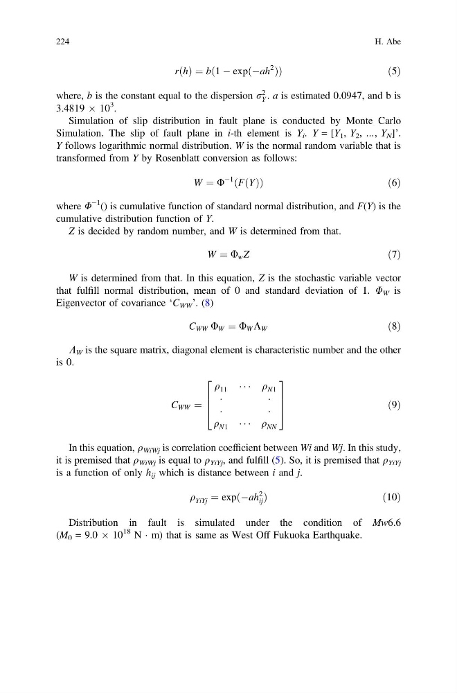
rðhÞ ¼ bð1 À expðÀah
2
ÞÞ
ð5Þ
where, b is the constant equal to the dispersion r
2
Y . a is estimated 0.0947, and b is
3.4819 Â 10
3 .
Simulation of slip distribution in fault plane is conducted by Monte Carlo
Simulation. The slip of fault plane in i-th element is Y i . Y = [Y 1 , Y 2 , …, Y N ]’.
Y follows logarithmic normal distribution. W is the normal random variable that is
transformed from Y by Rosenblatt conversion as follows:
W ¼ U
À1
ðFðYÞÞ
ð6Þ
where U
−1 () is cumulative function of standard normal distribution, and F(Y) is the
cumulative distribution function of Y.
Z is decided by random number, and W is determined from that.
W ¼ U w Z
ð7Þ
W is determined from that. In this equation, Z is the stochastic variable vector
that fulfill normal distribution, mean of 0 and standard deviation of 1. U W is
Eigenvector of covariance ‘C WW ’. (8)
C WW U W ¼ U W K W
ð8Þ
K W is the square matrix, diagonal element is characteristic number and the other
is 0.
C WW ¼
q 11 Á Á Á q N1
Á
Á
Á
Á
q N1 Á Á Á q NN
2
6
6
4
3
7
7
5
ð9Þ
In this equation, q WiWj is correlation coefficient between Wi and Wj. In this study,
it is premised that q WiWj is equal to q YiYj , and fulfill (5). So, it is premised that q YiYj
is a function of only h ij which is distance between i and j.
q YiYj ¼ expðÀah
2
ij Þ
ð 10Þ
Distribution in fault is simulated under the condition of Mw6.6
(M 0 = 9.0 Â 10
18 N Á m) that is same as West Off Fukuoka Earthquake.
224
H. Abe
2
ÞÞ
ð5Þ
where, b is the constant equal to the dispersion r
2
Y . a is estimated 0.0947, and b is
3.4819 Â 10
3 .
Simulation of slip distribution in fault plane is conducted by Monte Carlo
Simulation. The slip of fault plane in i-th element is Y i . Y = [Y 1 , Y 2 , …, Y N ]’.
Y follows logarithmic normal distribution. W is the normal random variable that is
transformed from Y by Rosenblatt conversion as follows:
W ¼ U
À1
ðFðYÞÞ
ð6Þ
where U
−1 () is cumulative function of standard normal distribution, and F(Y) is the
cumulative distribution function of Y.
Z is decided by random number, and W is determined from that.
W ¼ U w Z
ð7Þ
W is determined from that. In this equation, Z is the stochastic variable vector
that fulfill normal distribution, mean of 0 and standard deviation of 1. U W is
Eigenvector of covariance ‘C WW ’. (8)
C WW U W ¼ U W K W
ð8Þ
K W is the square matrix, diagonal element is characteristic number and the other
is 0.
C WW ¼
q 11 Á Á Á q N1
Á
Á
Á
Á
q N1 Á Á Á q NN
2
6
6
4
3
7
7
5
ð9Þ
In this equation, q WiWj is correlation coefficient between Wi and Wj. In this study,
it is premised that q WiWj is equal to q YiYj , and fulfill (5). So, it is premised that q YiYj
is a function of only h ij which is distance between i and j.
q YiYj ¼ expðÀah
2
ij Þ
ð 10Þ
Distribution in fault is simulated under the condition of Mw6.6
(M 0 = 9.0 Â 10
18 N Á m) that is same as West Off Fukuoka Earthquake.
224
H. Abe