

12 Phase Reconstruction with Iterated Hilbert Transforms
197
It is an observation of practice, that the latter approach based on the HT often
gives the most stable results. A reason for this is that the HT produces minimal
distortions to the signal’s spectrum. Indeed, all the methods mentioned are linear
transformations, which in Fourier space correspond to multiplications with factors
e
i , i, and i sign((), respectively. The factor for HT depends on frequency in a
“minimal” way, and does not have, contrary to the delay embedding, a parameter.
However, the HT provides only an approximate embedding, due to a mixing of phase
and amplitude modulations [13].
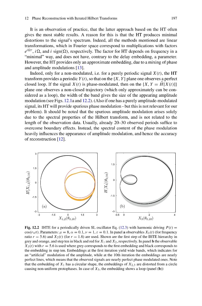
Indeed, only for a non-modulated, i.e. for a purely periodic signal X (t), the HT
transform provides a periodic Y (t), so that on the {X, Y } plane one observes a perfect
closed loop. If the signal X (t) is phase-modulated, then on the {X, Y = ˆ
H [X (t)]}
plane one observes a non-closed trajectory (which only approximately can be considered as a loop), the width of the band gives the size of the appearing amplitude
modulation (see Figs. 12.1a and 12.2). (Also if one has a purely amplitude-modulated
signal, its HT will provide spurious phase modulation - but this is not relevant for our
problem). It should be noted that the spurious amplitude modulation arises solely
due to the spectral properties of the Hilbert transform, and is not related to the
length of the observation data. Usually, already 20–30 observed periods suffice to
overcome boundary effects. Instead, the spectral content of the phase modulation
heavily influences the appearance of amplitude modulation, and hence the accuracy
of reconstruction [12].
-3
-1.5
0
1.5
3
-3
-1.5
0
1.5
3
-3
-1.5
0
1.5
-0.5
0
2
4
X 1,2 (θ 0,10 )
H[X
1,2 ](θ
0,10 )
X 3 (θ 0,10 )
H[X
3 ](θ
0,10 )
(a)
(b)
Fig. 12.2 IHTE for a periodically driven SL oscillator Eq. (12.3) with harmonic driving P(t) =
cos(r ωt). Parameters: μ = 8, α = 0.1, ν = 1, ε = 0.1. In panel a observables X 1 (t) (for frequency
ratio r = 5.6) and X 2 (t) (for r = 1.8) are used. Shown are the first step of the IHTE hierarchy in
grey and orange, and step ten in black and red for X 1 and X 2 , respectively. In panel b the observable
X 3 (t) with r = 5.6 is used where grey corresponds to the first embedding and black corresponds to
the embedding in step ten. Embeddings at the first iteration yield wide bands, which indicates for
an “artificial” modulation of the amplitude, while at the 10th iteration the embeddings are nearly
perfect lines, which means that the observed signals are nearly perfect phase modulated ones. Note
that the embedding of X 1 has a circular shape, the embeddings of X 2,3 are distorted from a circle
causing non-uniform protophases. In case of X 3 , the embedding shows a loop (panel (b))
197
It is an observation of practice, that the latter approach based on the HT often
gives the most stable results. A reason for this is that the HT produces minimal
distortions to the signal’s spectrum. Indeed, all the methods mentioned are linear
transformations, which in Fourier space correspond to multiplications with factors
e
i , i, and i sign((), respectively. The factor for HT depends on frequency in a
“minimal” way, and does not have, contrary to the delay embedding, a parameter.
However, the HT provides only an approximate embedding, due to a mixing of phase
and amplitude modulations [13].
Indeed, only for a non-modulated, i.e. for a purely periodic signal X (t), the HT
transform provides a periodic Y (t), so that on the {X, Y } plane one observes a perfect
closed loop. If the signal X (t) is phase-modulated, then on the {X, Y = ˆ
H [X (t)]}
plane one observes a non-closed trajectory (which only approximately can be considered as a loop), the width of the band gives the size of the appearing amplitude
modulation (see Figs. 12.1a and 12.2). (Also if one has a purely amplitude-modulated
signal, its HT will provide spurious phase modulation - but this is not relevant for our
problem). It should be noted that the spurious amplitude modulation arises solely
due to the spectral properties of the Hilbert transform, and is not related to the
length of the observation data. Usually, already 20–30 observed periods suffice to
overcome boundary effects. Instead, the spectral content of the phase modulation
heavily influences the appearance of amplitude modulation, and hence the accuracy
of reconstruction [12].
-3
-1.5
0
1.5
3
-3
-1.5
0
1.5
3
-3
-1.5
0
1.5
-0.5
0
2
4
X 1,2 (θ 0,10 )
H[X
1,2 ](θ
0,10 )
X 3 (θ 0,10 )
H[X
3 ](θ
0,10 )
(a)
(b)
Fig. 12.2 IHTE for a periodically driven SL oscillator Eq. (12.3) with harmonic driving P(t) =
cos(r ωt). Parameters: μ = 8, α = 0.1, ν = 1, ε = 0.1. In panel a observables X 1 (t) (for frequency
ratio r = 5.6) and X 2 (t) (for r = 1.8) are used. Shown are the first step of the IHTE hierarchy in
grey and orange, and step ten in black and red for X 1 and X 2 , respectively. In panel b the observable
X 3 (t) with r = 5.6 is used where grey corresponds to the first embedding and black corresponds to
the embedding in step ten. Embeddings at the first iteration yield wide bands, which indicates for
an “artificial” modulation of the amplitude, while at the 10th iteration the embeddings are nearly
perfect lines, which means that the observed signals are nearly perfect phase modulated ones. Note
that the embedding of X 1 has a circular shape, the embeddings of X 2,3 are distorted from a circle
causing non-uniform protophases. In case of X 3 , the embedding shows a loop (panel (b))