

164
A. Ben-Tal
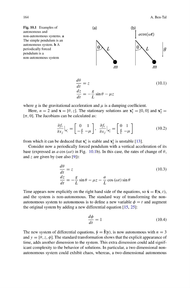
Fig. 10.1 Examples of
autonomous and
non-autonomous systems. a
The simple pendulum is an
autonomous system. b A
periodically forced
pendulum is a
non-autonomous system
a
dθ
dt
= z
(10.1)
dz
dt
= −
g
L
sin θ − μz
where g is the gravitational acceleration and μ is a damping coefficient.
Here, n = 2 and x = [θ, z]. The stationary solutions are x
∗
1 = [0, 0] and x
∗
2 =
[π, 0]. The Jacobians can be calculated as:
∂ f i
∂ x j
x
∗
1
=
0 1
−
g
L
−μ
,
∂ f i
∂ x j
x
∗
2
=
0 1
g
L
−μ
(10.2)
from which it can be deduced that x
∗
1 is stable and x
∗
2 is unstable [13].
Consider now a periodically forced pendulum with a vertical acceleration of its
base (expressed as a cos (ωt) in Fig. 10.1b). In this case, the rates of change of θ ,
and z are given by (see also [9]):
dθ
dt
= z
(10.3)
dz
dt
= −
g
L
sin θ − μz −
a
L
cos (ωt) sin θ
Time appears now explicitly on the right hand side of the equations, so ˙
x = f(x, t),
and the system is non-autonomous. The standard way of transforming the nonautonomous system to autonomous is to define a new variable φ = t and augment
the original system by adding a new differential equation [15, 25]:
dφ
dt
= 1
(10.4)
The new system of differential equations, ˙
y = ¯ f(y), is now autonomous with n = 3
and y = [θ, z, φ]. The standard transformation shows that the explicit appearance of
time, adds another dimension to the system. This extra dimension could add significant complexity to the behavior of solutions. In particular, a two dimensional nonautonomous system could exhibit chaos, whereas, a two-dimensional autonomous
A. Ben-Tal
Fig. 10.1 Examples of
autonomous and
non-autonomous systems. a
The simple pendulum is an
autonomous system. b A
periodically forced
pendulum is a
non-autonomous system
a
dθ
dt
= z
(10.1)
dz
dt
= −
g
L
sin θ − μz
where g is the gravitational acceleration and μ is a damping coefficient.
Here, n = 2 and x = [θ, z]. The stationary solutions are x
∗
1 = [0, 0] and x
∗
2 =
[π, 0]. The Jacobians can be calculated as:
∂ f i
∂ x j
x
∗
1
=
0 1
−
g
L
−μ
,
∂ f i
∂ x j
x
∗
2
=
0 1
g
L
−μ
(10.2)
from which it can be deduced that x
∗
1 is stable and x
∗
2 is unstable [13].
Consider now a periodically forced pendulum with a vertical acceleration of its
base (expressed as a cos (ωt) in Fig. 10.1b). In this case, the rates of change of θ ,
and z are given by (see also [9]):
dθ
dt
= z
(10.3)
dz
dt
= −
g
L
sin θ − μz −
a
L
cos (ωt) sin θ
Time appears now explicitly on the right hand side of the equations, so ˙
x = f(x, t),
and the system is non-autonomous. The standard way of transforming the nonautonomous system to autonomous is to define a new variable φ = t and augment
the original system by adding a new differential equation [15, 25]:
dφ
dt
= 1
(10.4)
The new system of differential equations, ˙
y = ¯ f(y), is now autonomous with n = 3
and y = [θ, z, φ]. The standard transformation shows that the explicit appearance of
time, adds another dimension to the system. This extra dimension could add significant complexity to the behavior of solutions. In particular, a two dimensional nonautonomous system could exhibit chaos, whereas, a two-dimensional autonomous