

124
J. M. I. Newman et al.
7.4.2 Analysis Based on Sect. 7.2
Assume k > a. Considering (7.7) over an arbitrary time-interval [0, T ] with T ≥
π
ω
,
the critical A-value A ∗ as defined in (7.4) is simply given by A ∗ = k − a. So as in
Sect. 7.2.4 we have the following: if A < k − a then, by the reasoning of Sect. 7.2.2,
the trajectories of (7.7) exhibit neutral stability; and if A > k − a then by the same
reasoning of Sect. 7.2.2, the trajectories of (7.7) exhibit stability.
As in Sect. 7.2.3, one can quantify the level of stability using the adiabatically
derived FTLE estimate defined in Eq. (7.2). If T is an integer multiple of
π
ω
then
this is given by
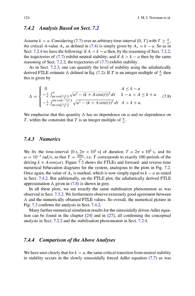
=
⎧
⎪ ⎪ ⎨
⎪ ⎪ ⎩
0
A ≤ k − a
−
1
π
π
arc cos(
a−k
A )
a 2 − (k + A cos(t)) 2 dt k − a < A ≤ k + a
−
1
π
arc cos(−
k+a
A )
arc cos(
a−k
A )
a 2 − (k + A cos(t)) 2 dt A > k + a.
(7.8)
We emphasise that this quantity has no dependence on ω and no dependence on
T , within the constraint that T is an integer multiple of
π
ω
.
7.4.3 Numerics
We fix the time-interval [0 s, 2π × 10
5 s] of duration T = 2π × 10
5 s, and fix
ω = 10
−3 rad/s, so that T =
200π
ω
, i.e. T corresponds to exactly 100 periods of the
driving k + A cos(ωt). Figure 7.3 shows the FTLEs and forward- and reverse-time
numerical bifurcation diagrams for the system, analogous to the plots in Fig. 7.2.
Once again, the value of A ∗ is marked, which is now simply equal to k − a as stated
in Sect. 7.4.2. But additionally, on the FTLE plot, the adiabatically derived FTLE
approximation given in (7.8) is shown in grey.
In all these plots, we see exactly the same stabilisation phenomenon as was
observed in Sect. 7.3.2. We furthermore observe extremely good agreement between
and the numerically obtained FTLE values. So overall, the numerical picture in
Fig. 7.3 confirms the analysis in Sect. 7.4.2.
Many further numerical simulation results for the sinusoidally driven Adler equation can be found in the chapter [24] and in [27], all confirming the conceptual
analysis in Sect. 7.2.2 and the stabilisation phenomenon in Sect. 7.2.4.
7.4.4 Comparison of the Above Analyses
We have seen clearly that for k > a, the same critical transition from neutral stability
to stability occurs in the slowly sinusoidally forced Adler equation (7.7) as was
J. M. I. Newman et al.
7.4.2 Analysis Based on Sect. 7.2
Assume k > a. Considering (7.7) over an arbitrary time-interval [0, T ] with T ≥
π
ω
,
the critical A-value A ∗ as defined in (7.4) is simply given by A ∗ = k − a. So as in
Sect. 7.2.4 we have the following: if A < k − a then, by the reasoning of Sect. 7.2.2,
the trajectories of (7.7) exhibit neutral stability; and if A > k − a then by the same
reasoning of Sect. 7.2.2, the trajectories of (7.7) exhibit stability.
As in Sect. 7.2.3, one can quantify the level of stability using the adiabatically
derived FTLE estimate defined in Eq. (7.2). If T is an integer multiple of
π
ω
then
this is given by
=
⎧
⎪ ⎪ ⎨
⎪ ⎪ ⎩
0
A ≤ k − a
−
1
π
π
arc cos(
a−k
A )
a 2 − (k + A cos(t)) 2 dt k − a < A ≤ k + a
−
1
π
arc cos(−
k+a
A )
arc cos(
a−k
A )
a 2 − (k + A cos(t)) 2 dt A > k + a.
(7.8)
We emphasise that this quantity has no dependence on ω and no dependence on
T , within the constraint that T is an integer multiple of
π
ω
.
7.4.3 Numerics
We fix the time-interval [0 s, 2π × 10
5 s] of duration T = 2π × 10
5 s, and fix
ω = 10
−3 rad/s, so that T =
200π
ω
, i.e. T corresponds to exactly 100 periods of the
driving k + A cos(ωt). Figure 7.3 shows the FTLEs and forward- and reverse-time
numerical bifurcation diagrams for the system, analogous to the plots in Fig. 7.2.
Once again, the value of A ∗ is marked, which is now simply equal to k − a as stated
in Sect. 7.4.2. But additionally, on the FTLE plot, the adiabatically derived FTLE
approximation given in (7.8) is shown in grey.
In all these plots, we see exactly the same stabilisation phenomenon as was
observed in Sect. 7.3.2. We furthermore observe extremely good agreement between
and the numerically obtained FTLE values. So overall, the numerical picture in
Fig. 7.3 confirms the analysis in Sect. 7.4.2.
Many further numerical simulation results for the sinusoidally driven Adler equation can be found in the chapter [24] and in [27], all confirming the conceptual
analysis in Sect. 7.2.2 and the stabilisation phenomenon in Sect. 7.2.4.
7.4.4 Comparison of the Above Analyses
We have seen clearly that for k > a, the same critical transition from neutral stability
to stability occurs in the slowly sinusoidally forced Adler equation (7.7) as was