

7 Non-asymptotic-time Dynamics
117
The above adiabatic reasoning is precisely the reasoning behind the stabilisation
phenomenon observed in Sect. 6.4.3 of the chapter [24]. Here in this chapter, we will
highlight how the stabilisation arising from this inherently finite-time reasoning does
not, in general, lend itself to being formalised and quantified in terms of traditional
long-time-asymptotic mathematical formalisms. This stands in contrast to the noiseinduced stability described in Sect. 6.4.2 of the chapter [24], the theory of which is
inherently tied to the model’s long-time-asymptotic dynamics.
7.2.3 Quantitative Rate of Synchronisation of Trajectories
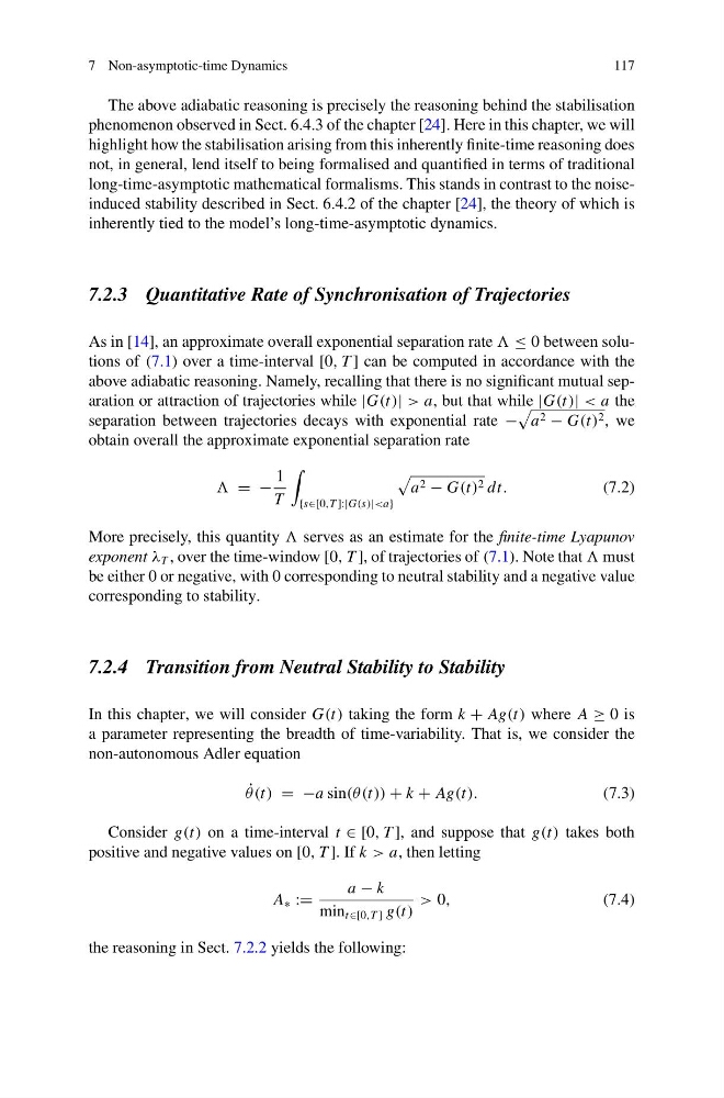
As in [14], an approximate overall exponential separation rate ≤ 0 between solutions of (7.1) over a time-interval [0, T ] can be computed in accordance with the
above adiabatic reasoning. Namely, recalling that there is no significant mutual separation or attraction of trajectories while |G(t)| > a, but that while |G(t)| < a the
separation between trajectories decays with exponential rate −
a 2 − G(t) 2 , we
obtain overall the approximate exponential separation rate
= −
1
T
{s∈[0,T ]:|G(s)|
(7.2)
More precisely, this quantity serves as an estimate for the finite-time Lyapunov
exponent λ T , over the time-window [0, T ], of trajectories of (7.1). Note that must
be either 0 or negative, with 0 corresponding to neutral stability and a negative value
corresponding to stability.
7.2.4 Transition from Neutral Stability to Stability
In this chapter, we will consider G(t) taking the form k + Ag(t) where A ≥ 0 is
a parameter representing the breadth of time-variability. That is, we consider the
non-autonomous Adler equation
˙
θ(t) = −a sin(θ (t)) + k + Ag(t).
(7.3)
Consider g(t) on a time-interval t ∈ [0, T ], and suppose that g(t) takes both
positive and negative values on [0, T ]. If k > a, then letting
A ∗ :=
a − k
min t∈[0,T ] g(t)
> 0,
(7.4)
the reasoning in Sect. 7.2.2 yields the following:
117
The above adiabatic reasoning is precisely the reasoning behind the stabilisation
phenomenon observed in Sect. 6.4.3 of the chapter [24]. Here in this chapter, we will
highlight how the stabilisation arising from this inherently finite-time reasoning does
not, in general, lend itself to being formalised and quantified in terms of traditional
long-time-asymptotic mathematical formalisms. This stands in contrast to the noiseinduced stability described in Sect. 6.4.2 of the chapter [24], the theory of which is
inherently tied to the model’s long-time-asymptotic dynamics.
7.2.3 Quantitative Rate of Synchronisation of Trajectories
As in [14], an approximate overall exponential separation rate ≤ 0 between solutions of (7.1) over a time-interval [0, T ] can be computed in accordance with the
above adiabatic reasoning. Namely, recalling that there is no significant mutual separation or attraction of trajectories while |G(t)| > a, but that while |G(t)| < a the
separation between trajectories decays with exponential rate −
a 2 − G(t) 2 , we
obtain overall the approximate exponential separation rate
= −
1
T
{s∈[0,T ]:|G(s)|
(7.2)
More precisely, this quantity serves as an estimate for the finite-time Lyapunov
exponent λ T , over the time-window [0, T ], of trajectories of (7.1). Note that must
be either 0 or negative, with 0 corresponding to neutral stability and a negative value
corresponding to stability.
7.2.4 Transition from Neutral Stability to Stability
In this chapter, we will consider G(t) taking the form k + Ag(t) where A ≥ 0 is
a parameter representing the breadth of time-variability. That is, we consider the
non-autonomous Adler equation
˙
θ(t) = −a sin(θ (t)) + k + Ag(t).
(7.3)
Consider g(t) on a time-interval t ∈ [0, T ], and suppose that g(t) takes both
positive and negative values on [0, T ]. If k > a, then letting
A ∗ :=
a − k
min t∈[0,T ] g(t)
> 0,
(7.4)
the reasoning in Sect. 7.2.2 yields the following: