

6 Synchronisation and Non-autonomicity
91
then the trajectory is unstable, i.e. exhibits sensitive dependence to changes in initial
condition; if λ max < 0 then the trajectory is stable against small perturbations; in the
intermediate case λ max = 0, the trajectory is said neutrally stable. The presence of
positive ALEs for the trajectories of a dynamical system is commonly accepted as
an indicator of chaos.
Two key assumptions of Definition (6.4) are that (i) the dynamical system being
analysed must be defined over infinite time and (ii) the formal limit t → ∞ in
Definition (6.4) exists. The first assumption can be satisfied by either an autonomous
system, or a non-autonomous system. Not all non-autonomous systems need be
defined over infinite time, however, as discussed in chapter [40] of this volume and
references therein. As for the second condition, Oseledets’ multiplicative ergodic
theorem [41] provides conditions for the existence of the limit, and hence of the
spectrum of ALEs described above. For an autonomous system, ALEs are typically
well-defined, but with some exceptions [42]. The same holds for non-autonomous
systems with simple forms of non-autonomicity such as periodic variation; but for
arbitrary aperiodic variation, the limit in Eq. (6.4) will typically not exist.
The ALE has the important property of being coordinate-invariant: it does not
depend on the choice of coordinates for the state space of the dynamical system.
6.3.1.2 Fourier Spectrum
The realisation of a physical process can be represented in the time domain, by a
time series, or in the frequency domain, e.g. by the Fourier spectrum of this time
series. The two representations give different insight into the underlying system, and
the frequency content of a time series is a precious tool to understand the system,
especially if it is oscillatory. A typical frequency domain representation is the discrete
Fourier transform (DFT) of a time series {x k } where the index k = 1, . . . , n represents
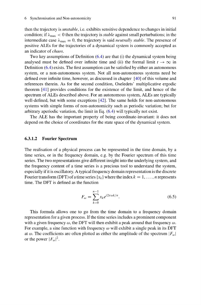
time. The DFT is defined as the function
F ω =
n−1
k=0
x k e
i2πωk/n
.
(6.5)
This formula allows one to go from the time domain to a frequency domain
representation for a given process. If the time series includes a prominent component
with a given frequency ω, the DFT will then exhibit a peak around that frequency ω.
For example, a sine function with frequency ω will exhibit a single peak in its DFT
at ω. The coefficients are often plotted as either the amplitude of the spectrum |F ω |
or the power |F ω |
2 .
91
then the trajectory is unstable, i.e. exhibits sensitive dependence to changes in initial
condition; if λ max < 0 then the trajectory is stable against small perturbations; in the
intermediate case λ max = 0, the trajectory is said neutrally stable. The presence of
positive ALEs for the trajectories of a dynamical system is commonly accepted as
an indicator of chaos.
Two key assumptions of Definition (6.4) are that (i) the dynamical system being
analysed must be defined over infinite time and (ii) the formal limit t → ∞ in
Definition (6.4) exists. The first assumption can be satisfied by either an autonomous
system, or a non-autonomous system. Not all non-autonomous systems need be
defined over infinite time, however, as discussed in chapter [40] of this volume and
references therein. As for the second condition, Oseledets’ multiplicative ergodic
theorem [41] provides conditions for the existence of the limit, and hence of the
spectrum of ALEs described above. For an autonomous system, ALEs are typically
well-defined, but with some exceptions [42]. The same holds for non-autonomous
systems with simple forms of non-autonomicity such as periodic variation; but for
arbitrary aperiodic variation, the limit in Eq. (6.4) will typically not exist.
The ALE has the important property of being coordinate-invariant: it does not
depend on the choice of coordinates for the state space of the dynamical system.
6.3.1.2 Fourier Spectrum
The realisation of a physical process can be represented in the time domain, by a
time series, or in the frequency domain, e.g. by the Fourier spectrum of this time
series. The two representations give different insight into the underlying system, and
the frequency content of a time series is a precious tool to understand the system,
especially if it is oscillatory. A typical frequency domain representation is the discrete
Fourier transform (DFT) of a time series {x k } where the index k = 1, . . . , n represents
time. The DFT is defined as the function
F ω =
n−1
k=0
x k e
i2πωk/n
.
(6.5)
This formula allows one to go from the time domain to a frequency domain
representation for a given process. If the time series includes a prominent component
with a given frequency ω, the DFT will then exhibit a peak around that frequency ω.
For example, a sine function with frequency ω will exhibit a single peak in its DFT
at ω. The coefficients are often plotted as either the amplitude of the spectrum |F ω |
or the power |F ω |
2 .