

84
H. Elnaggar et al.
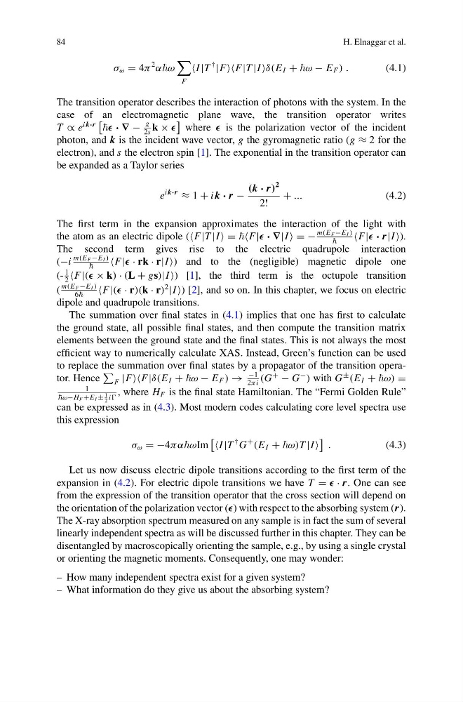
σ ω = 4π
2
αω
F
I |T
†
|FF|T |I δ(E I + ω − E F ) .
(4.1)
The transition operator describes the interaction of photons with the system. In the
case of an electromagnetic plane wave, the transition operator writes
T ∝ e
i k·r
· ∇ −
g
2s
k ×
where is the polarization vector of the incident
photon, and k is the incident wave vector, g the gyromagnetic ratio (g ≈ 2 for the
electron), and s the electron spin [1]. The exponential in the transition operator can
be expanded as a Taylor series
e
i k·r
≈ 1 + i k · r −
(k · r)
2
2!
+ ...
(4.2)
The first term in the expansion approximates the interaction of the light with
the atom as an electric dipole (F|T |I = F| · ∇|I = −
m(E F −E I )
F| · r|I ).
The second term gives rise to the electric quadrupole interaction
(−i
m(E F −E I )
F| · rk · r|I ) and to the (negligible) magnetic dipole one
(1
2
F|( × k) · (L + gs)|I ) [1], the third term is the octupole transition
(
m(E F −E I )
6
F|( · r)(k · r)
2
|I ) [2], and so on. In this chapter, we focus on electric
dipole and quadrupole transitions.
The summation over final states in (4.1) implies that one has first to calculate
the ground state, all possible final states, and then compute the transition matrix
elements between the ground state and the final states. This is not always the most
efficient way to numerically calculate XAS. Instead, Green’s function can be used
to replace the summation over final states by a propagator of the transition operator. Hence
F |FF|δ(E I + ω − E F ) →
−1
2πi
(G
+
− G
−
) with G
±
(E I + ω) =
1
ω−H F +E I ±
1
2 i
, where H F is the final state Hamiltonian. The “Fermi Golden Rule”
can be expressed as in (4.3). Most modern codes calculating core level spectra use
this expression
σ ω = −4παωIm
I |T
† G
+
(E I + ω)T |I
.
(4.3)
Let us now discuss electric dipole transitions according to the first term of the
expansion in (4.2). For electric dipole transitions we have T = · r. One can see
from the expression of the transition operator that the cross section will depend on
the orientation of the polarization vector () with respect to the absorbing system (r).
The X-ray absorption spectrum measured on any sample is in fact the sum of several
linearly independent spectra as will be discussed further in this chapter. They can be
disentangled by macroscopically orienting the sample, e.g., by using a single crystal
or orienting the magnetic moments. Consequently, one may wonder:
– How many independent spectra exist for a given system?
– What information do they give us about the absorbing system?
H. Elnaggar et al.
σ ω = 4π
2
αω
F
I |T
†
|FF|T |I δ(E I + ω − E F ) .
(4.1)
The transition operator describes the interaction of photons with the system. In the
case of an electromagnetic plane wave, the transition operator writes
T ∝ e
i k·r
· ∇ −
g
2s
k ×
where is the polarization vector of the incident
photon, and k is the incident wave vector, g the gyromagnetic ratio (g ≈ 2 for the
electron), and s the electron spin [1]. The exponential in the transition operator can
be expanded as a Taylor series
e
i k·r
≈ 1 + i k · r −
(k · r)
2
2!
+ ...
(4.2)
The first term in the expansion approximates the interaction of the light with
the atom as an electric dipole (F|T |I = F| · ∇|I = −
m(E F −E I )
F| · r|I ).
The second term gives rise to the electric quadrupole interaction
(−i
m(E F −E I )
F| · rk · r|I ) and to the (negligible) magnetic dipole one
(1
2
F|( × k) · (L + gs)|I ) [1], the third term is the octupole transition
(
m(E F −E I )
6
F|( · r)(k · r)
2
|I ) [2], and so on. In this chapter, we focus on electric
dipole and quadrupole transitions.
The summation over final states in (4.1) implies that one has first to calculate
the ground state, all possible final states, and then compute the transition matrix
elements between the ground state and the final states. This is not always the most
efficient way to numerically calculate XAS. Instead, Green’s function can be used
to replace the summation over final states by a propagator of the transition operator. Hence
F |FF|δ(E I + ω − E F ) →
−1
2πi
(G
+
− G
−
) with G
±
(E I + ω) =
1
ω−H F +E I ±
1
2 i
, where H F is the final state Hamiltonian. The “Fermi Golden Rule”
can be expressed as in (4.3). Most modern codes calculating core level spectra use
this expression
σ ω = −4παωIm
I |T
† G
+
(E I + ω)T |I
.
(4.3)
Let us now discuss electric dipole transitions according to the first term of the
expansion in (4.2). For electric dipole transitions we have T = · r. One can see
from the expression of the transition operator that the cross section will depend on
the orientation of the polarization vector () with respect to the absorbing system (r).
The X-ray absorption spectrum measured on any sample is in fact the sum of several
linearly independent spectra as will be discussed further in this chapter. They can be
disentangled by macroscopically orienting the sample, e.g., by using a single crystal
or orienting the magnetic moments. Consequently, one may wonder:
– How many independent spectra exist for a given system?
– What information do they give us about the absorbing system?