

72
P. Krüger
where |m are excited states with energy E m and η is an infinitesimal positive number.
The exact eigenstates and energies of the interacting electron systems are unknown,
so (3.22) cannot be evaluated directly. For a non-interacting electron gas, however,
all eigenstates are Slater determinants, and (3.22) can be calculated. The only excitations which give non-zero matrix elements are single particle–hole excitations
|m = c
+
p c h |0 with energy p − h , where p and h label states above and below the
Fermi level, respectively. This gives the response function in the independent particle
approximation
χ 0 (r, r
, ω) =
hp
φ
∗
h (r)φ p (r)φ
∗
p (r
)φ h (r
)
ω − p + h + iη
− [p ↔ h] .
(3.23)
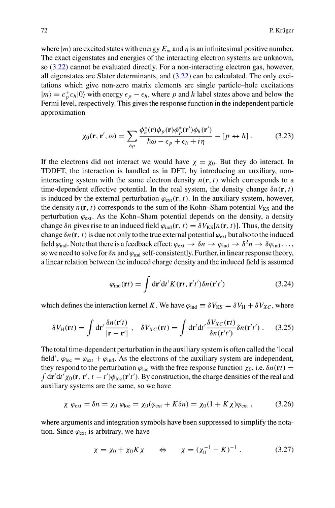
If the electrons did not interact we would have χ = χ 0 . But they do interact. In
TDDFT, the interaction is handled as in DFT, by introducing an auxiliary, noninteracting system with the same electron density n(r, t) which corresponds to a
time-dependent effective potential. In the real system, the density change δn(r, t)
is induced by the external perturbation ϕ ext (r, t). In the auxiliary system, however,
the density n(r, t) corresponds to the sum of the Kohn–Sham potential V KS and the
perturbation ϕ ext . As the Kohn–Sham potential depends on the density, a density
change δn gives rise to an induced field ϕ ind (r, t) = δV KS [n(r, t)]. Thus, the density
change δn(r, t) is due not only to the true external potential ϕ ext but also to the induced
field ϕ ind . Note that there is a feedback effect: ϕ ext → δn → ϕ ind → δ
2 n → δϕ ind . . . ,
so we need to solve for δn and ϕ ind self-consistently. Further, in linear response theory,
a linear relation between the induced charge density and the induced field is assumed
ϕ ind (rt) =
dr
dt
K (rt, r
t
)δn(r
t
)
(3.24)
which defines the interaction kernel K . We have ϕ ind ≡ δV KS = δV H + δV XC , where
δV H (rt) =
dr
δn(r
t)
|r − r |
, δV XC (rt) =
dr
dt
δV XC (rt)
δn(r t )
δn(r
t
) . (3.25)
The total time-dependent perturbation in the auxiliary system is often called the ‘local
field’, ϕ loc = ϕ ext + ϕ ind . As the electrons of the auxiliary system are independent,
they respond to the perturbation ϕ loc with the free response function χ 0 , i.e. δn(rt) =
dr
dt
χ 0 (r, r
, t − t
)φ loc (r
t
). By construction, the charge densities of the real and
auxiliary systems are the same, so we have
χ ϕ ext = δn = χ 0 ϕ loc = χ 0 (ϕ ext + K δn) = χ 0 (1 + K χ)ϕ ext ,
(3.26)
where arguments and integration symbols have been suppressed to simplify the notation. Since ϕ ext is arbitrary, we have
χ = χ 0 + χ 0 K χ
⇔
χ = (χ
−1
0 − K )
−1
.
(3.27)
P. Krüger
where |m are excited states with energy E m and η is an infinitesimal positive number.
The exact eigenstates and energies of the interacting electron systems are unknown,
so (3.22) cannot be evaluated directly. For a non-interacting electron gas, however,
all eigenstates are Slater determinants, and (3.22) can be calculated. The only excitations which give non-zero matrix elements are single particle–hole excitations
|m = c
+
p c h |0 with energy p − h , where p and h label states above and below the
Fermi level, respectively. This gives the response function in the independent particle
approximation
χ 0 (r, r
, ω) =
hp
φ
∗
h (r)φ p (r)φ
∗
p (r
)φ h (r
)
ω − p + h + iη
− [p ↔ h] .
(3.23)
If the electrons did not interact we would have χ = χ 0 . But they do interact. In
TDDFT, the interaction is handled as in DFT, by introducing an auxiliary, noninteracting system with the same electron density n(r, t) which corresponds to a
time-dependent effective potential. In the real system, the density change δn(r, t)
is induced by the external perturbation ϕ ext (r, t). In the auxiliary system, however,
the density n(r, t) corresponds to the sum of the Kohn–Sham potential V KS and the
perturbation ϕ ext . As the Kohn–Sham potential depends on the density, a density
change δn gives rise to an induced field ϕ ind (r, t) = δV KS [n(r, t)]. Thus, the density
change δn(r, t) is due not only to the true external potential ϕ ext but also to the induced
field ϕ ind . Note that there is a feedback effect: ϕ ext → δn → ϕ ind → δ
2 n → δϕ ind . . . ,
so we need to solve for δn and ϕ ind self-consistently. Further, in linear response theory,
a linear relation between the induced charge density and the induced field is assumed
ϕ ind (rt) =
dr
dt
K (rt, r
t
)δn(r
t
)
(3.24)
which defines the interaction kernel K . We have ϕ ind ≡ δV KS = δV H + δV XC , where
δV H (rt) =
dr
δn(r
t)
|r − r |
, δV XC (rt) =
dr
dt
δV XC (rt)
δn(r t )
δn(r
t
) . (3.25)
The total time-dependent perturbation in the auxiliary system is often called the ‘local
field’, ϕ loc = ϕ ext + ϕ ind . As the electrons of the auxiliary system are independent,
they respond to the perturbation ϕ loc with the free response function χ 0 , i.e. δn(rt) =
dr
dt
χ 0 (r, r
, t − t
)φ loc (r
t
). By construction, the charge densities of the real and
auxiliary systems are the same, so we have
χ ϕ ext = δn = χ 0 ϕ loc = χ 0 (ϕ ext + K δn) = χ 0 (1 + K χ)ϕ ext ,
(3.26)
where arguments and integration symbols have been suppressed to simplify the notation. Since ϕ ext is arbitrary, we have
χ = χ 0 + χ 0 K χ
⇔
χ = (χ
−1
0 − K )
−1
.
(3.27)