

66
L. Wugang et al.
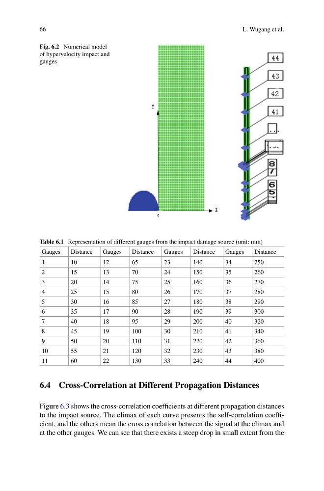
Fig. 6.2 Numerical model
of hypervelocity impact and
gauges
Table 6.1 Representation of different gauges from the impact damage source (unit: mm)
Gauges
Distance
Gauges
Distance
Gauges
Distance
Gauges
Distance
1
10
12
65
23
140
34
250
2
15
13
70
24
150
35
260
3
20
14
75
25
160
36
270
4
25
15
80
26
170
37
280
5
30
16
85
27
180
38
290
6
35
17
90
28
190
39
300
7
40
18
95
29
200
40
320
8
45
19
100
30
210
41
340
9
50
20
110
31
220
42
360
10
55
21
120
32
230
43
380
11
60
22
130
33
240
44
400
6.4 Cross-Correlation at Different Propagation Distances
Figure 6.3 shows the cross-correlation coefficients at different propagation distances
to the impact source. The climax of each curve presents the self-correlation coefficient, and the others mean the cross correlation between the signal at the climax and
at the other gauges. We can see that there exists a steep drop in small extent from the
L. Wugang et al.
Fig. 6.2 Numerical model
of hypervelocity impact and
gauges
Table 6.1 Representation of different gauges from the impact damage source (unit: mm)
Gauges
Distance
Gauges
Distance
Gauges
Distance
Gauges
Distance
1
10
12
65
23
140
34
250
2
15
13
70
24
150
35
260
3
20
14
75
25
160
36
270
4
25
15
80
26
170
37
280
5
30
16
85
27
180
38
290
6
35
17
90
28
190
39
300
7
40
18
95
29
200
40
320
8
45
19
100
30
210
41
340
9
50
20
110
31
220
42
360
10
55
21
120
32
230
43
380
11
60
22
130
33
240
44
400
6.4 Cross-Correlation at Different Propagation Distances
Figure 6.3 shows the cross-correlation coefficients at different propagation distances
to the impact source. The climax of each curve presents the self-correlation coefficient, and the others mean the cross correlation between the signal at the climax and
at the other gauges. We can see that there exists a steep drop in small extent from the