

10 Prediction of Residual Life of Oil and Gas Pipeline Corrosion …
107
Enter
The simplest
feature
The most
complicated
feature
Map with
features
Output
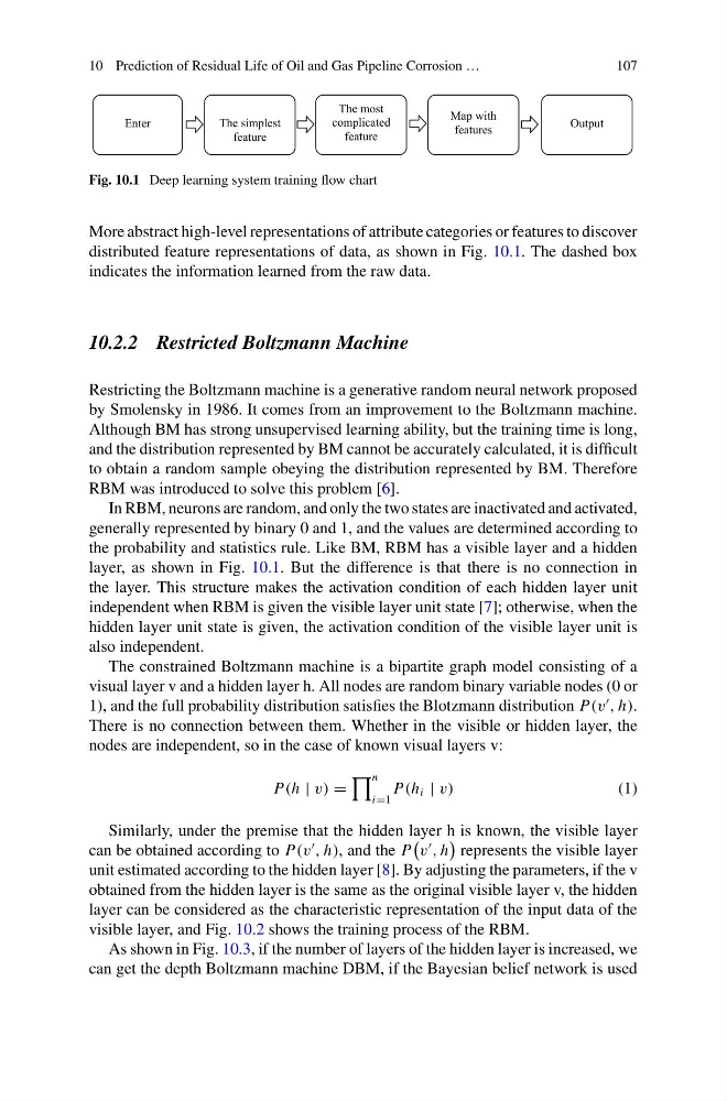
Fig. 10.1 Deep learning system training flow chart
More abstract high-level representations of attribute categories or features to discover
distributed feature representations of data, as shown in Fig. 10.1. The dashed box
indicates the information learned from the raw data.
10.2.2 Restricted Boltzmann Machine
Restricting the Boltzmann machine is a generative random neural network proposed
by Smolensky in 1986. It comes from an improvement to the Boltzmann machine.
Although BM has strong unsupervised learning ability, but the training time is long,
and the distribution represented by BM cannot be accurately calculated, it is difficult
to obtain a random sample obeying the distribution represented by BM. Therefore
RBM was introduced to solve this problem [6].
In RBM, neurons are random, and only the two states are inactivated and activated,
generally represented by binary 0 and 1, and the values are determined according to
the probability and statistics rule. Like BM, RBM has a visible layer and a hidden
layer, as shown in Fig. 10.1. But the difference is that there is no connection in
the layer. This structure makes the activation condition of each hidden layer unit
independent when RBM is given the visible layer unit state [7]; otherwise, when the
hidden layer unit state is given, the activation condition of the visible layer unit is
also independent.
The constrained Boltzmann machine is a bipartite graph model consisting of a
visual layer v and a hidden layer h. All nodes are random binary variable nodes (0 or
1), and the full probability distribution satisfies the Blotzmann distribution P(v
, h).
There is no connection between them. Whether in the visible or hidden layer, the
nodes are independent, so in the case of known visual layers v:
P(h | v) =
n
i=1
P(h i | v)
(1)
Similarly, under the premise that the hidden layer h is known, the visible layer
can be obtained according to P(v
, h), and the P
v
, h
represents the visible layer
unit estimated according to the hidden layer [8]. By adjusting the parameters, if the v
obtained from the hidden layer is the same as the original visible layer v, the hidden
layer can be considered as the characteristic representation of the input data of the
visible layer, and Fig. 10.2 shows the training process of the RBM.
As shown in Fig. 10.3, if the number of layers of the hidden layer is increased, we
can get the depth Boltzmann machine DBM, if the Bayesian belief network is used
107
Enter
The simplest
feature
The most
complicated
feature
Map with
features
Output
Fig. 10.1 Deep learning system training flow chart
More abstract high-level representations of attribute categories or features to discover
distributed feature representations of data, as shown in Fig. 10.1. The dashed box
indicates the information learned from the raw data.
10.2.2 Restricted Boltzmann Machine
Restricting the Boltzmann machine is a generative random neural network proposed
by Smolensky in 1986. It comes from an improvement to the Boltzmann machine.
Although BM has strong unsupervised learning ability, but the training time is long,
and the distribution represented by BM cannot be accurately calculated, it is difficult
to obtain a random sample obeying the distribution represented by BM. Therefore
RBM was introduced to solve this problem [6].
In RBM, neurons are random, and only the two states are inactivated and activated,
generally represented by binary 0 and 1, and the values are determined according to
the probability and statistics rule. Like BM, RBM has a visible layer and a hidden
layer, as shown in Fig. 10.1. But the difference is that there is no connection in
the layer. This structure makes the activation condition of each hidden layer unit
independent when RBM is given the visible layer unit state [7]; otherwise, when the
hidden layer unit state is given, the activation condition of the visible layer unit is
also independent.
The constrained Boltzmann machine is a bipartite graph model consisting of a
visual layer v and a hidden layer h. All nodes are random binary variable nodes (0 or
1), and the full probability distribution satisfies the Blotzmann distribution P(v
, h).
There is no connection between them. Whether in the visible or hidden layer, the
nodes are independent, so in the case of known visual layers v:
P(h | v) =
n
i=1
P(h i | v)
(1)
Similarly, under the premise that the hidden layer h is known, the visible layer
can be obtained according to P(v
, h), and the P
v
, h
represents the visible layer
unit estimated according to the hidden layer [8]. By adjusting the parameters, if the v
obtained from the hidden layer is the same as the original visible layer v, the hidden
layer can be considered as the characteristic representation of the input data of the
visible layer, and Fig. 10.2 shows the training process of the RBM.
As shown in Fig. 10.3, if the number of layers of the hidden layer is increased, we
can get the depth Boltzmann machine DBM, if the Bayesian belief network is used