

68
3 Area-Preserving Maps
and
U i−1 = B i−2 T i−1 B
−1
i−2 .
(3.42)
If we next note that in the limit i → ∞, B i → B ∗ , where B is defined in Eq. (3.37),
then in the limit i → ∞, Eqs. (3.41) and (3.42) take the form
T
∗
= B
∗ T
∗ U
∗ B
∗−1 ,
(3.43)
U
∗
= B
∗ T
∗ B
∗−1 .
(3.44)
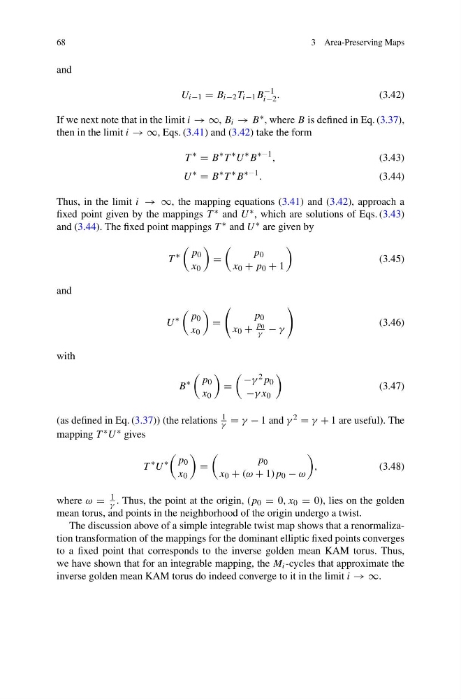
Thus, in the limit i → ∞, the mapping equations (3.41) and (3.42), approach a
fixed point given by the mappings T ∗ and U ∗ , which are solutions of Eqs. (3.43)
and (3.44). The fixed point mappings T ∗ and U ∗ are given by
T
∗
p 0
x 0
=
p 0
x 0 + p 0 + 1
(3.45)
and
U
∗
p 0
x 0
=
p 0
x 0 +
p 0
γ − γ
(3.46)
with
B
∗
p 0
x 0
=
−γ 2 p 0
−γ x 0
(3.47)
(as defined in Eq. (3.37)) (the relations
1
γ = γ − 1 and γ 2 = γ + 1 are useful). The
mapping T ∗ U ∗ gives
T
∗ U
∗
p 0
x 0
=
p 0
x 0 + (ω + 1)p 0 − ω
,
(3.48)
where ω =
1
γ . Thus, the point at the origin, (p 0 = 0, x 0 = 0), lies on the golden
mean torus, and points in the neighborhood of the origin undergo a twist.
The discussion above of a simple integrable twist map shows that a renormalization transformation of the mappings for the dominant elliptic fixed points converges
to a fixed point that corresponds to the inverse golden mean KAM torus. Thus,
we have shown that for an integrable mapping, the M i -cycles that approximate the
inverse golden mean KAM torus do indeed converge to it in the limit i → ∞.
3 Area-Preserving Maps
and
U i−1 = B i−2 T i−1 B
−1
i−2 .
(3.42)
If we next note that in the limit i → ∞, B i → B ∗ , where B is defined in Eq. (3.37),
then in the limit i → ∞, Eqs. (3.41) and (3.42) take the form
T
∗
= B
∗ T
∗ U
∗ B
∗−1 ,
(3.43)
U
∗
= B
∗ T
∗ B
∗−1 .
(3.44)
Thus, in the limit i → ∞, the mapping equations (3.41) and (3.42), approach a
fixed point given by the mappings T ∗ and U ∗ , which are solutions of Eqs. (3.43)
and (3.44). The fixed point mappings T ∗ and U ∗ are given by
T
∗
p 0
x 0
=
p 0
x 0 + p 0 + 1
(3.45)
and
U
∗
p 0
x 0
=
p 0
x 0 +
p 0
γ − γ
(3.46)
with
B
∗
p 0
x 0
=
−γ 2 p 0
−γ x 0
(3.47)
(as defined in Eq. (3.37)) (the relations
1
γ = γ − 1 and γ 2 = γ + 1 are useful). The
mapping T ∗ U ∗ gives
T
∗ U
∗
p 0
x 0
=
p 0
x 0 + (ω + 1)p 0 − ω
,
(3.48)
where ω =
1
γ . Thus, the point at the origin, (p 0 = 0, x 0 = 0), lies on the golden
mean torus, and points in the neighborhood of the origin undergo a twist.
The discussion above of a simple integrable twist map shows that a renormalization transformation of the mappings for the dominant elliptic fixed points converges
to a fixed point that corresponds to the inverse golden mean KAM torus. Thus,
we have shown that for an integrable mapping, the M i -cycles that approximate the
inverse golden mean KAM torus do indeed converge to it in the limit i → ∞.