

480
F Gaussian Ensembles
where
¯
G N =
⎛
⎜
⎜
⎜
⎜
⎜
⎝
φ 0 (1)
φ 0 (2) ... φ 0 (N)
φ 1 (1)
φ 1 (2) ... φ 1 (N)
φ 2 (1)
φ 2 (2) ... φ 2 (N)
. . .
. . .
. . .
. . .
φ N −1 (1) φ N −1 (2) . . . φ N −1 (N)
⎞
⎟
⎟
⎟
⎟
⎟
⎠
,
(F.69)
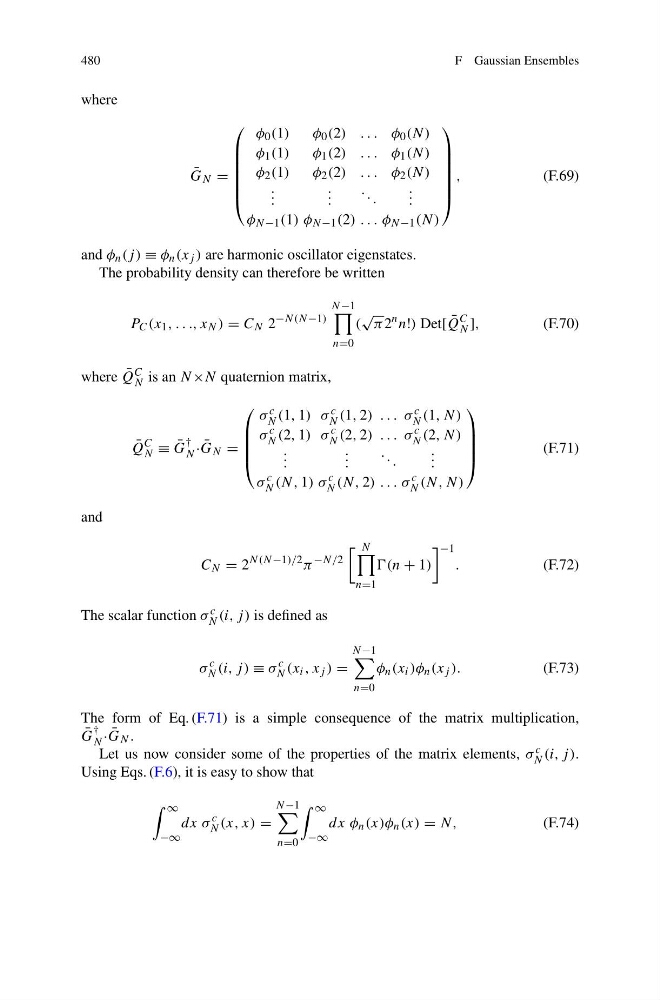
and φ n (j ) ≡ φ n (x j ) are harmonic oscillator eigenstates.
The probability density can therefore be written
P C (x 1 , . . ., x N ) = C N 2
−N(N−1)
N −1
n=0
(
√
π 2
n n!) Det[ ¯
Q
C
N ],
(F.70)
where ¯
Q C
N is an N ×N quaternion matrix,
¯
Q
C
N ≡ ¯
G
†
N · ¯
G N =
⎛
⎜
⎜
⎜
⎝
σ c
N (1, 1) σ c
N (1, 2) . . . σ c
N (1, N)
σ c
N (2, 1) σ c
N (2, 2) . . . σ c
N (2, N)
. . .
. . .
. . .
. . .
σ c
N (N, 1) σ c
N (N, 2) . . . σ c
N (N, N)
⎞
⎟
⎟
⎟
⎠
(F.71)
and
C N = 2
N(N−1)/2 π
−N/2
N
n=1
(n + 1)
−1
.
(F.72)
The scalar function σ c
N (i, j ) is defined as
σ
c
N (i, j ) ≡ σ
c
N (x i , x j ) =
N −1
n=0
φ n (x i )φ n (x j ).
(F.73)
The form of Eq. (F.71) is a simple consequence of the matrix multiplication,
¯
G
†
N · ¯
G N .
Let us now consider some of the properties of the matrix elements, σ c
N (i, j ).
Using Eqs. (F.6), it is easy to show that
∞
−∞
dx σ
c
N (x, x) =
N −1
n=0
∞
−∞
dx φ n (x)φ n (x) = N,
(F.74)
F Gaussian Ensembles
where
¯
G N =
⎛
⎜
⎜
⎜
⎜
⎜
⎝
φ 0 (1)
φ 0 (2) ... φ 0 (N)
φ 1 (1)
φ 1 (2) ... φ 1 (N)
φ 2 (1)
φ 2 (2) ... φ 2 (N)
. . .
. . .
. . .
. . .
φ N −1 (1) φ N −1 (2) . . . φ N −1 (N)
⎞
⎟
⎟
⎟
⎟
⎟
⎠
,
(F.69)
and φ n (j ) ≡ φ n (x j ) are harmonic oscillator eigenstates.
The probability density can therefore be written
P C (x 1 , . . ., x N ) = C N 2
−N(N−1)
N −1
n=0
(
√
π 2
n n!) Det[ ¯
Q
C
N ],
(F.70)
where ¯
Q C
N is an N ×N quaternion matrix,
¯
Q
C
N ≡ ¯
G
†
N · ¯
G N =
⎛
⎜
⎜
⎜
⎝
σ c
N (1, 1) σ c
N (1, 2) . . . σ c
N (1, N)
σ c
N (2, 1) σ c
N (2, 2) . . . σ c
N (2, N)
. . .
. . .
. . .
. . .
σ c
N (N, 1) σ c
N (N, 2) . . . σ c
N (N, N)
⎞
⎟
⎟
⎟
⎠
(F.71)
and
C N = 2
N(N−1)/2 π
−N/2
N
n=1
(n + 1)
−1
.
(F.72)
The scalar function σ c
N (i, j ) is defined as
σ
c
N (i, j ) ≡ σ
c
N (x i , x j ) =
N −1
n=0
φ n (x i )φ n (x j ).
(F.73)
The form of Eq. (F.71) is a simple consequence of the matrix multiplication,
¯
G
†
N · ¯
G N .
Let us now consider some of the properties of the matrix elements, σ c
N (i, j ).
Using Eqs. (F.6), it is easy to show that
∞
−∞
dx σ
c
N (x, x) =
N −1
n=0
∞
−∞
dx φ n (x)φ n (x) = N,
(F.74)