

2.6 KAM Theory
35
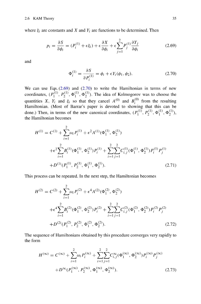
where ξ i are constants and X and Y i are functions to be determined. Then
p i =
∂S
∂φ i
= (P
(1)
i + ξ i ) +
∂X
∂φ i
+
2
j =1
P
(1)
j
∂Y j
∂φ i
(2.69)
and
(1)
i =
∂S
∂P
(1)
i
= φ i + Y i (φ 1 , φ 2 ).
(2.70)
We can use Eqs. (2.69) and (2.70) to write the Hamiltonian in terms of new
coordinates, (P
(1)
1 , P
(1)
2 , ,
(1)
1 , ,
(1)
2 ). The idea of Kolmogorov was to choose the
quantities X, Y i and ξ i so that they cancel A (0) and B
(0)
i
from the resulting
Hamiltonian. (Most of Barrar’s paper is devoted to showing that this can be
done.) Then, in terms of the new canonical coordinates, (P
(1)
1 , P
(1)
2 , ,
(1)
1 , ,
(1)
2 ),
the Hamiltonian becomes
H
(1)
= C
(1)
+
2
i=1
ω i P
(1)
i +
2 A
(1) ((
(1)
1 , ,
(1)
2 )
+
2
2
i=1
B
(1)
i ((
(1)
1 , ,
(1)
2 )P
(1)
i +
2
i=1
2
j =1
C
(1)
i,j ((
(1)
1 , ,
(1)
2 )P
(1)
i P
(1)
j
+D
(1) (P
(1)
1 , P
(1)
2 , ,
(1)
1 , ,
(1)
2 ).
(2.71)
This process can be repeated. In the next step, the Hamiltonian becomes
H
(2)
= C
(2)
+
2
i=1
ω i P
(2)
i +
4 A
(2) ((
(2)
1 , ,
(2)
2 )
+
4
2
i=1
B
(2)
i ((
(2)
1 , ,
(2)
2 )P
(2)
i +
2
i=1
2
j =1
C
(2)
i,j ((
(2)
1 , ,
(2)
2 )P
(2)
i P
(2)
j
+D
(2) (P
(2)
1 , P
(2)
2 , ,
(2)
1 , ,
(2)
2 ).
(2.72)
The sequence of Hamiltonians obtained by this procedure converges very rapidly to
the form
H
(∞)
= C
(∞)
+
2
i=1
ω i P
(∞)
i
+
2
i=1
2
j =1
C
∞
i,j ((
(∞)
1 , ,
(∞)
2 )P
(∞)
i
P
(∞)
j
+D
∞ (P
(∞)
1
, P
(∞)
2
, ,
(∞)
1 , ,
(∞)
2 ).
(2.73)
35
where ξ i are constants and X and Y i are functions to be determined. Then
p i =
∂S
∂φ i
= (P
(1)
i + ξ i ) +
∂X
∂φ i
+
2
j =1
P
(1)
j
∂Y j
∂φ i
(2.69)
and
(1)
i =
∂S
∂P
(1)
i
= φ i + Y i (φ 1 , φ 2 ).
(2.70)
We can use Eqs. (2.69) and (2.70) to write the Hamiltonian in terms of new
coordinates, (P
(1)
1 , P
(1)
2 , ,
(1)
1 , ,
(1)
2 ). The idea of Kolmogorov was to choose the
quantities X, Y i and ξ i so that they cancel A (0) and B
(0)
i
from the resulting
Hamiltonian. (Most of Barrar’s paper is devoted to showing that this can be
done.) Then, in terms of the new canonical coordinates, (P
(1)
1 , P
(1)
2 , ,
(1)
1 , ,
(1)
2 ),
the Hamiltonian becomes
H
(1)
= C
(1)
+
2
i=1
ω i P
(1)
i +
2 A
(1) ((
(1)
1 , ,
(1)
2 )
+
2
2
i=1
B
(1)
i ((
(1)
1 , ,
(1)
2 )P
(1)
i +
2
i=1
2
j =1
C
(1)
i,j ((
(1)
1 , ,
(1)
2 )P
(1)
i P
(1)
j
+D
(1) (P
(1)
1 , P
(1)
2 , ,
(1)
1 , ,
(1)
2 ).
(2.71)
This process can be repeated. In the next step, the Hamiltonian becomes
H
(2)
= C
(2)
+
2
i=1
ω i P
(2)
i +
4 A
(2) ((
(2)
1 , ,
(2)
2 )
+
4
2
i=1
B
(2)
i ((
(2)
1 , ,
(2)
2 )P
(2)
i +
2
i=1
2
j =1
C
(2)
i,j ((
(2)
1 , ,
(2)
2 )P
(2)
i P
(2)
j
+D
(2) (P
(2)
1 , P
(2)
2 , ,
(2)
1 , ,
(2)
2 ).
(2.72)
The sequence of Hamiltonians obtained by this procedure converges very rapidly to
the form
H
(∞)
= C
(∞)
+
2
i=1
ω i P
(∞)
i
+
2
i=1
2
j =1
C
∞
i,j ((
(∞)
1 , ,
(∞)
2 )P
(∞)
i
P
(∞)
j
+D
∞ (P
(∞)
1
, P
(∞)
2
, ,
(∞)
1 , ,
(∞)
2 ).
(2.73)