

446
D Invariant Measures
D.3.4 General Formula for Invariant Measure of Unitary
Matrices
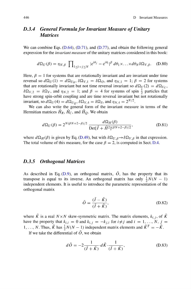
We can combine Eqs. (D.64), (D.71), and (D.77), and obtain the following general
expression for the invariant measure of the unitary matrices considered in this book:
dd U (β) = η N,β
1≤i
iθ j − e
iθ i |
β dθ 1 ×. . .×dθ N δδ V ,β . (D.80)
Here, β = 1 for systems that are rotationally invariant and are invariant under time
reversal so dd U (1) = dd U R , δδ V ,1 = δδ O , and η N,1 = 1; β = 2 for systems
that are rotationally invariant but not time reversal invariant so dd U (2) = dd U C ,
δδ V ,2 = δδ V , and η N,2 = 1; and β = 4 for systems of spin
1
2 particles that
have strong spin-orbit coupling and are time reversal invariant but not rotationally
invariant, so dd U (4) = dd U Q , δδ V ,4 = δδ S , and η N,4 = 2 N/2 .
We can also write the general form of the invariant measure in terms of the
Hermitian matrices ¯
H R , ¯
H C , and ¯
H Q . We obtain
dd U (β) = 2
N(βN+2−β)/2
dd H (β)
Det[ ¯
I + ¯
H 2 ] (βN +2−β)/2 ,
(D.81)
where dd H (β) is given by Eq. (D.49), but with δδ U,β →δδ V ,β in that expression.
The total volume of this measure, for the case β = 2, is computed in Sect. D.4.
D.3.5 Orthogonal Matrices
As described in Eq. (D.9), an orthogonal matrix, ¯
O, has the property that its
transpose is equal to its inverse. An orthogonal matrix has only
1
2 N(N − 1)
independent elements. It is useful to introduce the parametric representation of the
orthogonal matrix
¯
O =
( ¯
I − ¯
K)
( ¯
I + ¯
K)
,
(D.82)
where ¯
K is a real N×N skew-symmetric matrix. The matrix elements, k i,j , of ¯
K
have the property that k i,i = 0 and k i,j = −k j,i for i =j and i = 1, . . ., N, j =
1, . . ., N. Thus, ¯
K has
1
2 N(N − 1) independent matrix elements and ¯
K T = − ¯
K.
If we take the differential of ¯
O, we obtain
d ¯
O = −2
1
( ¯
I + ¯
K)
·d ¯
K·
1
( ¯
I + ¯
K)
,
(D.83)
D Invariant Measures
D.3.4 General Formula for Invariant Measure of Unitary
Matrices
We can combine Eqs. (D.64), (D.71), and (D.77), and obtain the following general
expression for the invariant measure of the unitary matrices considered in this book:
dd U (β) = η N,β
1≤i
iθ j − e
iθ i |
β dθ 1 ×. . .×dθ N δδ V ,β . (D.80)
Here, β = 1 for systems that are rotationally invariant and are invariant under time
reversal so dd U (1) = dd U R , δδ V ,1 = δδ O , and η N,1 = 1; β = 2 for systems
that are rotationally invariant but not time reversal invariant so dd U (2) = dd U C ,
δδ V ,2 = δδ V , and η N,2 = 1; and β = 4 for systems of spin
1
2 particles that
have strong spin-orbit coupling and are time reversal invariant but not rotationally
invariant, so dd U (4) = dd U Q , δδ V ,4 = δδ S , and η N,4 = 2 N/2 .
We can also write the general form of the invariant measure in terms of the
Hermitian matrices ¯
H R , ¯
H C , and ¯
H Q . We obtain
dd U (β) = 2
N(βN+2−β)/2
dd H (β)
Det[ ¯
I + ¯
H 2 ] (βN +2−β)/2 ,
(D.81)
where dd H (β) is given by Eq. (D.49), but with δδ U,β →δδ V ,β in that expression.
The total volume of this measure, for the case β = 2, is computed in Sect. D.4.
D.3.5 Orthogonal Matrices
As described in Eq. (D.9), an orthogonal matrix, ¯
O, has the property that its
transpose is equal to its inverse. An orthogonal matrix has only
1
2 N(N − 1)
independent elements. It is useful to introduce the parametric representation of the
orthogonal matrix
¯
O =
( ¯
I − ¯
K)
( ¯
I + ¯
K)
,
(D.82)
where ¯
K is a real N×N skew-symmetric matrix. The matrix elements, k i,j , of ¯
K
have the property that k i,i = 0 and k i,j = −k j,i for i =j and i = 1, . . ., N, j =
1, . . ., N. Thus, ¯
K has
1
2 N(N − 1) independent matrix elements and ¯
K T = − ¯
K.
If we take the differential of ¯
O, we obtain
d ¯
O = −2
1
( ¯
I + ¯
K)
·d ¯
K·
1
( ¯
I + ¯
K)
,
(D.83)