

28
2 Fundamental Concepts
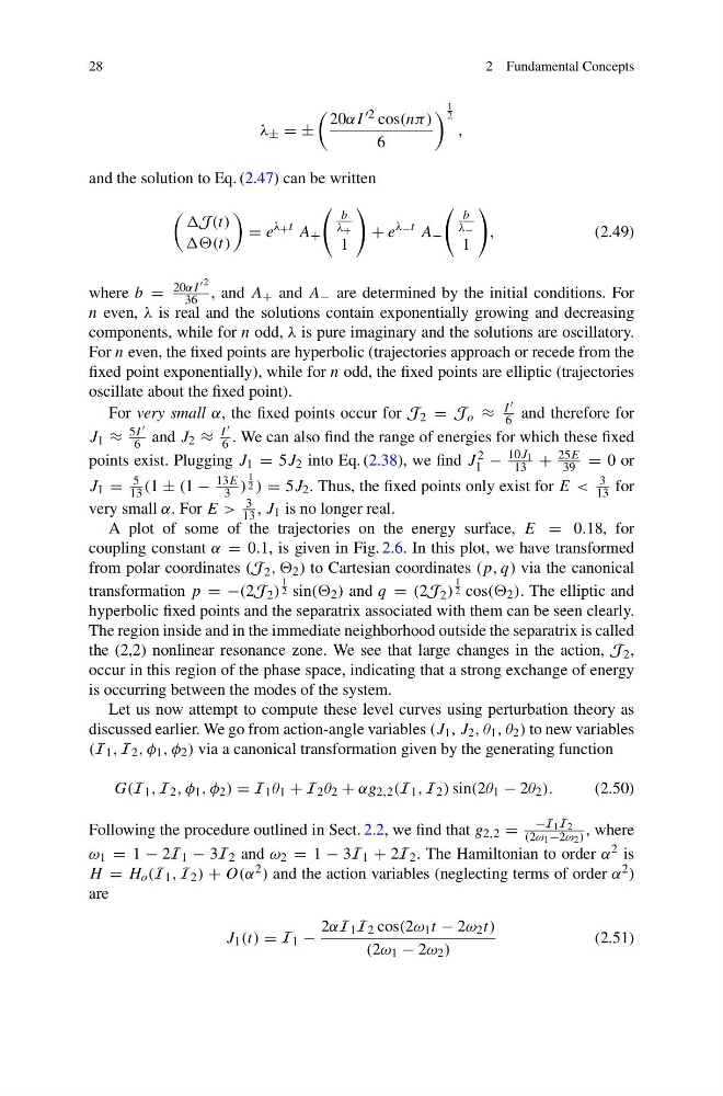
λ ± = ±
20αI 2 cos(nπ )
6
1
2
,
and the solution to Eq. (2.47) can be written
J(t)
= e
λ + t A +
b
λ +
1
+ e
λ − t A −
b
λ −
1
,
(2.49)
where b =
20αI 2
36 , and A + and A − are determined by the initial conditions. For
n even, λ is real and the solutions contain exponentially growing and decreasing
components, while for n odd, λ is pure imaginary and the solutions are oscillatory.
For n even, the fixed points are hyperbolic (trajectories approach or recede from the
fixed point exponentially), while for n odd, the fixed points are elliptic (trajectories
oscillate about the fixed point).
For very small α, the fixed points occur for J 2 = J o ≈
I
6 and therefore for
J 1 ≈
5I
6 and J 2 ≈
I
6 . We can also find the range of energies for which these fixed
points exist. Plugging J 1 = 5J 2 into Eq. (2.38), we find J 2
1 −
10J 1
13 +
25E
39 = 0 or
J 1 =
5
13 (1 ± (1 −
13E
3 )
1
2 ) = 5J 2 . Thus, the fixed points only exist for E <
3
13 for
very small α. For E >
3
13 , J 1 is no longer real.
A plot of some of the trajectories on the energy surface, E = 0.18, for
coupling constant α = 0.1, is given in Fig. 2.6. In this plot, we have transformed
from polar coordinates (J 2 , , 2 ) to Cartesian coordinates (p, q) via the canonical
transformation p = −(2J 2 )
1
2 sin(( 2 ) and q = (2J 2 )
1
2 cos(( 2 ). The elliptic and
hyperbolic fixed points and the separatrix associated with them can be seen clearly.
The region inside and in the immediate neighborhood outside the separatrix is called
the (2,2) nonlinear resonance zone. We see that large changes in the action, J 2 ,
occur in this region of the phase space, indicating that a strong exchange of energy
is occurring between the modes of the system.
Let us now attempt to compute these level curves using perturbation theory as
discussed earlier. We go from action-angle variables (J 1 , J 2 , θ 1 , θ 2 ) to new variables
(I 1 , I 2 , φ 1 , φ 2 ) via a canonical transformation given by the generating function
G(I 1 , I 2 , φ 1 , φ 2 ) = I 1 θ 1 + I 2 θ 2 + αg 2,2 (I 1 , I 2 ) sin(2θ 1 − 2θ 2 ).
(2.50)
Following the procedure outlined in Sect. 2.2, we find that g 2,2 =
−I 1 I 2
(2ω 1 −2ω 2 ) , where
ω 1 = 1 − 2I 1 − 3I 2 and ω 2 = 1 − 3I 1 + 2I 2 . The Hamiltonian to order α 2 is
H = H o (I 1 , I 2 ) + O(α 2 ) and the action variables (neglecting terms of order α 2 )
are
J 1 (t) = I 1 −
2αI 1 I 2 cos(2ω 1 t − 2ω 2 t)
(2ω 1 − 2ω 2 )
(2.51)
2 Fundamental Concepts
λ ± = ±
20αI 2 cos(nπ )
6
1
2
,
and the solution to Eq. (2.47) can be written
J(t)
= e
λ + t A +
b
λ +
1
+ e
λ − t A −
b
λ −
1
,
(2.49)
where b =
20αI 2
36 , and A + and A − are determined by the initial conditions. For
n even, λ is real and the solutions contain exponentially growing and decreasing
components, while for n odd, λ is pure imaginary and the solutions are oscillatory.
For n even, the fixed points are hyperbolic (trajectories approach or recede from the
fixed point exponentially), while for n odd, the fixed points are elliptic (trajectories
oscillate about the fixed point).
For very small α, the fixed points occur for J 2 = J o ≈
I
6 and therefore for
J 1 ≈
5I
6 and J 2 ≈
I
6 . We can also find the range of energies for which these fixed
points exist. Plugging J 1 = 5J 2 into Eq. (2.38), we find J 2
1 −
10J 1
13 +
25E
39 = 0 or
J 1 =
5
13 (1 ± (1 −
13E
3 )
1
2 ) = 5J 2 . Thus, the fixed points only exist for E <
3
13 for
very small α. For E >
3
13 , J 1 is no longer real.
A plot of some of the trajectories on the energy surface, E = 0.18, for
coupling constant α = 0.1, is given in Fig. 2.6. In this plot, we have transformed
from polar coordinates (J 2 , , 2 ) to Cartesian coordinates (p, q) via the canonical
transformation p = −(2J 2 )
1
2 sin(( 2 ) and q = (2J 2 )
1
2 cos(( 2 ). The elliptic and
hyperbolic fixed points and the separatrix associated with them can be seen clearly.
The region inside and in the immediate neighborhood outside the separatrix is called
the (2,2) nonlinear resonance zone. We see that large changes in the action, J 2 ,
occur in this region of the phase space, indicating that a strong exchange of energy
is occurring between the modes of the system.
Let us now attempt to compute these level curves using perturbation theory as
discussed earlier. We go from action-angle variables (J 1 , J 2 , θ 1 , θ 2 ) to new variables
(I 1 , I 2 , φ 1 , φ 2 ) via a canonical transformation given by the generating function
G(I 1 , I 2 , φ 1 , φ 2 ) = I 1 θ 1 + I 2 θ 2 + αg 2,2 (I 1 , I 2 ) sin(2θ 1 − 2θ 2 ).
(2.50)
Following the procedure outlined in Sect. 2.2, we find that g 2,2 =
−I 1 I 2
(2ω 1 −2ω 2 ) , where
ω 1 = 1 − 2I 1 − 3I 2 and ω 2 = 1 − 3I 1 + 2I 2 . The Hamiltonian to order α 2 is
H = H o (I 1 , I 2 ) + O(α 2 ) and the action variables (neglecting terms of order α 2 )
are
J 1 (t) = I 1 −
2αI 1 I 2 cos(2ω 1 t − 2ω 2 t)
(2ω 1 − 2ω 2 )
(2.51)