

346
10 Time-Periodic Quantum Systems
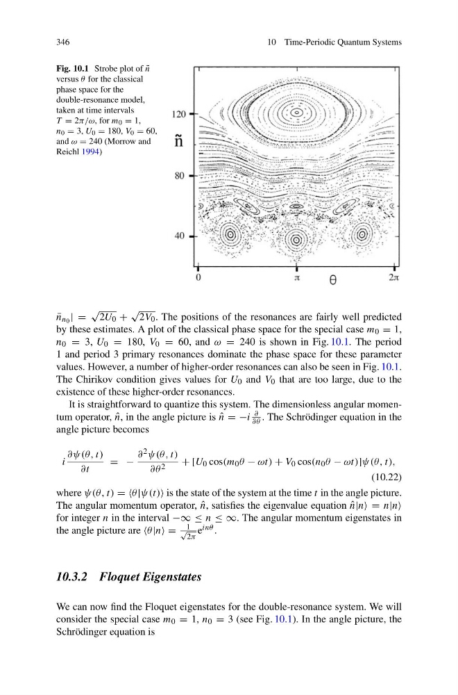
Fig. 10.1 Strobe plot of ˜
n
versus θ for the classical
phase space for the
double-resonance model,
taken at time intervals
T = 2π/ω, for m 0 = 1,
n 0 = 3, U 0 = 180, V 0 = 60,
and ω = 240 (Morrow and
Reichl 1994)
¯
n n 0 | =
√
2U 0 +
√
2V 0 . The positions of the resonances are fairly well predicted
by these estimates. A plot of the classical phase space for the special case m 0 = 1,
n 0 = 3, U 0 = 180, V 0 = 60, and ω = 240 is shown in Fig. 10.1. The period
1 and period 3 primary resonances dominate the phase space for these parameter
values. However, a number of higher-order resonances can also be seen in Fig. 10.1.
The Chirikov condition gives values for U 0 and V 0 that are too large, due to the
existence of these higher-order resonances.
It is straightforward to quantize this system. The dimensionless angular momentum operator, ˆ
n, in the angle picture is ˆ
n = −i
∂
∂θ . The Schrödinger equation in the
angle picture becomes
i
∂ψ(θ, t)
∂t
= −
∂ 2 ψ(θ, t)
∂θ 2
+ [U 0 cos(m 0 θ − ωt) + V 0 cos(n 0 θ − ωt)]ψ(θ, t),
(10.22)
where ψ(θ, t) = =θ |ψ(t) is the state of the system at the time t in the angle picture.
The angular momentum operator, ˆ
n, satisfies the eigenvalue equation ˆ
n|n = n|n
for integer n in the interval −∞ ≤ n ≤ ∞. The angular momentum eigenstates in
the angle picture are |n =
1
√
2π
e inθ .
10.3.2 Floquet Eigenstates
We can now find the Floquet eigenstates for the double-resonance system. We will
consider the special case m 0 = 1, n 0 = 3 (see Fig. 10.1). In the angle picture, the
Schrödinger equation is
10 Time-Periodic Quantum Systems
Fig. 10.1 Strobe plot of ˜
n
versus θ for the classical
phase space for the
double-resonance model,
taken at time intervals
T = 2π/ω, for m 0 = 1,
n 0 = 3, U 0 = 180, V 0 = 60,
and ω = 240 (Morrow and
Reichl 1994)
¯
n n 0 | =
√
2U 0 +
√
2V 0 . The positions of the resonances are fairly well predicted
by these estimates. A plot of the classical phase space for the special case m 0 = 1,
n 0 = 3, U 0 = 180, V 0 = 60, and ω = 240 is shown in Fig. 10.1. The period
1 and period 3 primary resonances dominate the phase space for these parameter
values. However, a number of higher-order resonances can also be seen in Fig. 10.1.
The Chirikov condition gives values for U 0 and V 0 that are too large, due to the
existence of these higher-order resonances.
It is straightforward to quantize this system. The dimensionless angular momentum operator, ˆ
n, in the angle picture is ˆ
n = −i
∂
∂θ . The Schrödinger equation in the
angle picture becomes
i
∂ψ(θ, t)
∂t
= −
∂ 2 ψ(θ, t)
∂θ 2
+ [U 0 cos(m 0 θ − ωt) + V 0 cos(n 0 θ − ωt)]ψ(θ, t),
(10.22)
where ψ(θ, t) = =θ |ψ(t) is the state of the system at the time t in the angle picture.
The angular momentum operator, ˆ
n, satisfies the eigenvalue equation ˆ
n|n = n|n
for integer n in the interval −∞ ≤ n ≤ ∞. The angular momentum eigenstates in
the angle picture are |n =
1
√
2π
e inθ .
10.3.2 Floquet Eigenstates
We can now find the Floquet eigenstates for the double-resonance system. We will
consider the special case m 0 = 1, n 0 = 3 (see Fig. 10.1). In the angle picture, the
Schrödinger equation is