

322
9 Semiclassical Theory: Path Integrals
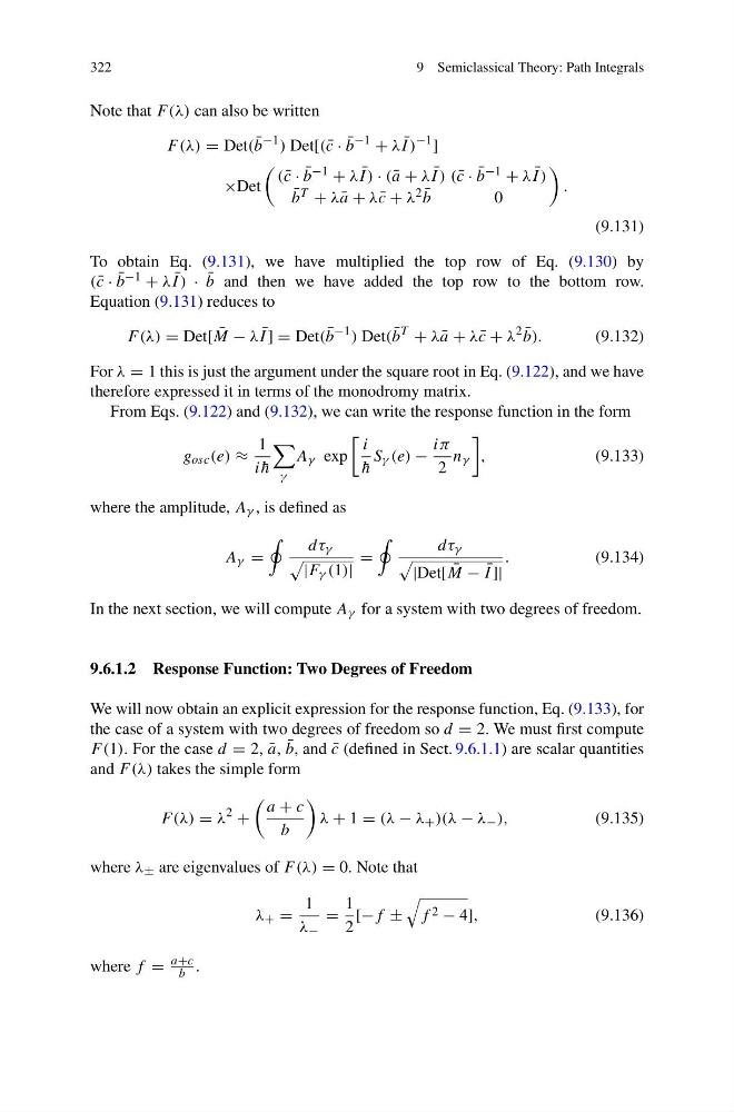
Note that F (λ) can also be written
F (λ) = Det( ¯
b
−1 ) Det[( ¯
c · ¯
b
−1
+ λ ¯
I )
−1
]
×Det
( ¯
c · ¯
b −1 + λ ¯
I ) · ( ¯
a + λ ¯
I ) ( ¯
c · ¯
b −1 + λ ¯
I )
¯
b T + λ ¯
a + λ ¯
c + λ 2 ¯
b
0
.
(9.131)
To obtain Eq. (9.131), we have multiplied the top row of Eq. (9.130) by
( ¯
c · ¯
b −1 + λ ¯
I ) · ¯
b and then we have added the top row to the bottom row.
Equation (9.131) reduces to
F (λ) = Det[ ¯
M − λ ¯
I ] = Det( ¯
b
−1 ) Det( ¯
b
T
+ λ ¯
a + λ ¯
c + λ
2 ¯
b).
(9.132)
For λ = 1 this is just the argument under the square root in Eq. (9.122), and we have
therefore expressed it in terms of the monodromy matrix.
From Eqs. (9.122) and (9.132), we can write the response function in the form
g osc (e) ≈
1
i ¯
h
γ
A γ exp
i
¯
h
S γ (e) −
iπ
2
n γ
,
(9.133)
where the amplitude, A γ , is defined as
A γ =
dτ γ
|F γ (1)|
=
dτ γ
|Det[ ¯
M − ¯
I ]|
.
(9.134)
In the next section, we will compute A γ for a system with two degrees of freedom.
9.6.1.2 Response Function: Two Degrees of Freedom
We will now obtain an explicit expression for the response function, Eq. (9.133), for
the case of a system with two degrees of freedom so d = 2. We must first compute
F (1). For the case d = 2, ¯
a, ¯
b, and ¯
c (defined in Sect. 9.6.1.1) are scalar quantities
and F (λ) takes the simple form
F (λ) = λ
2
+
a + c
b
λ + 1 = (λ − λ + )(λ − λ − ),
(9.135)
where λ ± are eigenvalues of F (λ) = 0. Note that
λ + =
1
λ −
=
1
2
[−f ±
f 2 − 4],
(9.136)
where f =
a+c
b .
9 Semiclassical Theory: Path Integrals
Note that F (λ) can also be written
F (λ) = Det( ¯
b
−1 ) Det[( ¯
c · ¯
b
−1
+ λ ¯
I )
−1
]
×Det
( ¯
c · ¯
b −1 + λ ¯
I ) · ( ¯
a + λ ¯
I ) ( ¯
c · ¯
b −1 + λ ¯
I )
¯
b T + λ ¯
a + λ ¯
c + λ 2 ¯
b
0
.
(9.131)
To obtain Eq. (9.131), we have multiplied the top row of Eq. (9.130) by
( ¯
c · ¯
b −1 + λ ¯
I ) · ¯
b and then we have added the top row to the bottom row.
Equation (9.131) reduces to
F (λ) = Det[ ¯
M − λ ¯
I ] = Det( ¯
b
−1 ) Det( ¯
b
T
+ λ ¯
a + λ ¯
c + λ
2 ¯
b).
(9.132)
For λ = 1 this is just the argument under the square root in Eq. (9.122), and we have
therefore expressed it in terms of the monodromy matrix.
From Eqs. (9.122) and (9.132), we can write the response function in the form
g osc (e) ≈
1
i ¯
h
γ
A γ exp
i
¯
h
S γ (e) −
iπ
2
n γ
,
(9.133)
where the amplitude, A γ , is defined as
A γ =
dτ γ
|F γ (1)|
=
dτ γ
|Det[ ¯
M − ¯
I ]|
.
(9.134)
In the next section, we will compute A γ for a system with two degrees of freedom.
9.6.1.2 Response Function: Two Degrees of Freedom
We will now obtain an explicit expression for the response function, Eq. (9.133), for
the case of a system with two degrees of freedom so d = 2. We must first compute
F (1). For the case d = 2, ¯
a, ¯
b, and ¯
c (defined in Sect. 9.6.1.1) are scalar quantities
and F (λ) takes the simple form
F (λ) = λ
2
+
a + c
b
λ + 1 = (λ − λ + )(λ − λ − ),
(9.135)
where λ ± are eigenvalues of F (λ) = 0. Note that
λ + =
1
λ −
=
1
2
[−f ±
f 2 − 4],
(9.136)
where f =
a+c
b .