

Weighted Hurwitz Numbers, τ -Functions, and Matrix Integrals
85
−k +1 − k +2
···
···
N
N+1
−
1
βc
−
1
βc
− 1
···
···
−
1
βc
−
1
βc
− 1
···
···
Re s = N +
1
2
Re s = N +
1
2
C k
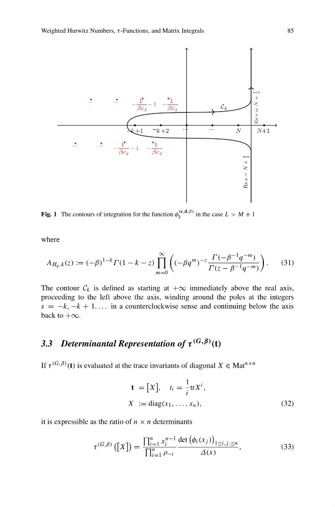
Fig. 1 The contours of integration for the function φ
(c,d,β)
k
in the case L > M + 1
where
A H q ,k (z) := (−β)
1−k Γ (1 − k − z)
∞
m=0
(−βq
m )
−z Γ (−β −1 q −m )
Γ (z − β −1 q −m )
.
(31)
The contour C k is defined as starting at +∞ immediately above the real axis,
proceeding to the left above the axis, winding around the poles at the integers
s = −k, −k + 1. . . . in a counterclockwise sense and continuing below the axis
back to +∞.
3.3 Determinantal Representation of τ (G,β) (t)
If τ (G,β) (t) is evaluated at the trace invariants of diagonal X ∈ Mat
n×n
t =
X
, t i =
1
i
trX
i ,
X := diag(x 1 , . . . , x n ),
(32)
it is expressible as the ratio of n × n determinants
τ
(G,β)
X
=
n
i=1 x
n−1
i
n
i=1 ρ −i
det
φ i (x j )
1≤i,j,≤n
Δ(x)
,
(33)
85
−k +1 − k +2
···
···
N
N+1
−
1
βc
−
1
βc
− 1
···
···
−
1
βc
−
1
βc
− 1
···
···
Re s = N +
1
2
Re s = N +
1
2
C k
Fig. 1 The contours of integration for the function φ
(c,d,β)
k
in the case L > M + 1
where
A H q ,k (z) := (−β)
1−k Γ (1 − k − z)
∞
m=0
(−βq
m )
−z Γ (−β −1 q −m )
Γ (z − β −1 q −m )
.
(31)
The contour C k is defined as starting at +∞ immediately above the real axis,
proceeding to the left above the axis, winding around the poles at the integers
s = −k, −k + 1. . . . in a counterclockwise sense and continuing below the axis
back to +∞.
3.3 Determinantal Representation of τ (G,β) (t)
If τ (G,β) (t) is evaluated at the trace invariants of diagonal X ∈ Mat
n×n
t =
X
, t i =
1
i
trX
i ,
X := diag(x 1 , . . . , x n ),
(32)
it is expressible as the ratio of n × n determinants
τ
(G,β)
X
=
n
i=1 x
n−1
i
n
i=1 ρ −i
det
φ i (x j )
1≤i,j,≤n
Δ(x)
,
(33)