

Fast Tests for Probing the Causal Structure of Quantum Processes
623
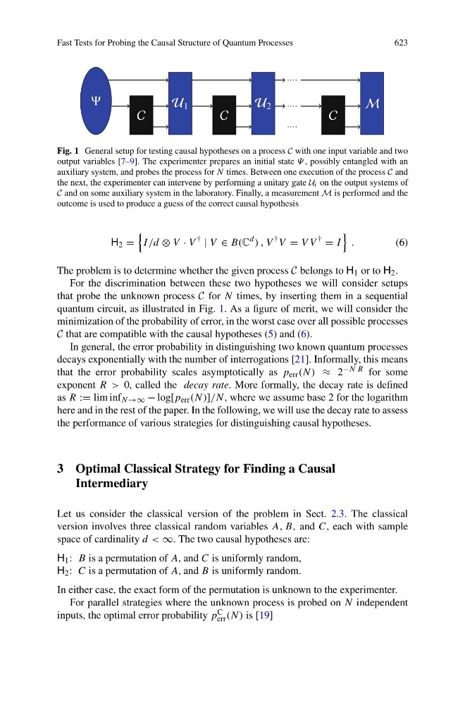
Fig. 1 General setup for testing causal hypotheses on a process C with one input variable and two
output variables [7–9]. The experimenter prepares an initial state Ψ , possibly entangled with an
auxiliary system, and probes the process for N times. Between one execution of the process C and
the next, the experimenter can intervene by performing a unitary gate U i on the output systems of
C and on some auxiliary system in the laboratory. Finally, a measurement M is performed and the
outcome is used to produce a guess of the correct causal hypothesis
H 2 =
I/d ⊗ V · V
†
| V ∈ B(C
d ) , V
† V = V V
†
= I
.
(6)
The problem is to determine whether the given process C belongs to H 1 or to H 2 .
For the discrimination between these two hypotheses we will consider setups
that probe the unknown process C for N times, by inserting them in a sequential
quantum circuit, as illustrated in Fig. 1. As a figure of merit, we will consider the
minimization of the probability of error, in the worst case over all possible processes
C that are compatible with the causal hypotheses (5) and (6).
In general, the error probability in distinguishing two known quantum processes
decays exponentially with the number of interrogations [21]. Informally, this means
that the error probability scales asymptotically as p err (N) ≈ 2 −N R for some
exponent R > 0, called the decay rate. More formally, the decay rate is defined
as R := lim inf N →∞ − log[p err (N)]/N , where we assume base 2 for the logarithm
here and in the rest of the paper. In the following, we will use the decay rate to assess
the performance of various strategies for distinguishing causal hypotheses.
3 Optimal Classical Strategy for Finding a Causal
Intermediary
Let us consider the classical version of the problem in Sect. 2.3. The classical
version involves three classical random variables A, B, and C, each with sample
space of cardinality d < ∞. The two causal hypotheses are:
H 1 : B is a permutation of A, and C is uniformly random,
H 2 : C is a permutation of A, and B is uniformly random.
In either case, the exact form of the permutation is unknown to the experimenter.
For parallel strategies where the unknown process is probed on N independent
inputs, the optimal error probability p C
err (N) is [19]
623
Fig. 1 General setup for testing causal hypotheses on a process C with one input variable and two
output variables [7–9]. The experimenter prepares an initial state Ψ , possibly entangled with an
auxiliary system, and probes the process for N times. Between one execution of the process C and
the next, the experimenter can intervene by performing a unitary gate U i on the output systems of
C and on some auxiliary system in the laboratory. Finally, a measurement M is performed and the
outcome is used to produce a guess of the correct causal hypothesis
H 2 =
I/d ⊗ V · V
†
| V ∈ B(C
d ) , V
† V = V V
†
= I
.
(6)
The problem is to determine whether the given process C belongs to H 1 or to H 2 .
For the discrimination between these two hypotheses we will consider setups
that probe the unknown process C for N times, by inserting them in a sequential
quantum circuit, as illustrated in Fig. 1. As a figure of merit, we will consider the
minimization of the probability of error, in the worst case over all possible processes
C that are compatible with the causal hypotheses (5) and (6).
In general, the error probability in distinguishing two known quantum processes
decays exponentially with the number of interrogations [21]. Informally, this means
that the error probability scales asymptotically as p err (N) ≈ 2 −N R for some
exponent R > 0, called the decay rate. More formally, the decay rate is defined
as R := lim inf N →∞ − log[p err (N)]/N , where we assume base 2 for the logarithm
here and in the rest of the paper. In the following, we will use the decay rate to assess
the performance of various strategies for distinguishing causal hypotheses.
3 Optimal Classical Strategy for Finding a Causal
Intermediary
Let us consider the classical version of the problem in Sect. 2.3. The classical
version involves three classical random variables A, B, and C, each with sample
space of cardinality d < ∞. The two causal hypotheses are:
H 1 : B is a permutation of A, and C is uniformly random,
H 2 : C is a permutation of A, and B is uniformly random.
In either case, the exact form of the permutation is unknown to the experimenter.
For parallel strategies where the unknown process is probed on N independent
inputs, the optimal error probability p C
err (N) is [19]