

Darboux-Bäcklund Transformations for Spin-Valued Linear Problems
43
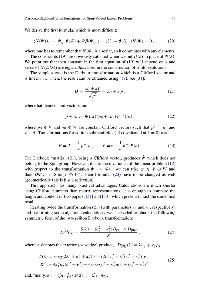
We derive the first formula, which is most difficult:
(N(Ψ )), μ = Ψ, μ β β β(Ψ ) + Ψ β β β(Ψ, μ ) = (U μ + β β β(U μ ))N(Ψ ) = 0 ,
(20)
where one has to remember that N(Ψ ) is a scalar, so it commutes with any elements.
The constraints (19) are obviously satisfied when we put D(λ) in place of Ψ (λ).
We point out that then constant in the first equation of (19) will depend on λ and
zeros of N(D(λ)) are eigenvalues used in the construction of soliton solutions.
The simplest case is the Darboux transformation which is a Clifford vector and
is linear in λ. Then, the result can be obtained using (17), see [31]:
D =
λn + κp
p 2
= λ ˆ
n + κ ˆ
p ,
(21)
where hat denotes unit vectors and
p + in := Ψ (iκ)(p 0 + in 0 )Ψ
−1 (iκ) ,
(22)
where p 0 ∈ V and n 0 ∈ W are constant Clifford vectors such that p 2
0 = n 2
0 and
κ ∈ R. Transformations for soliton submanifolds (14) (evaluated at λ = 0) read
˜
F = F +
1
κ
ˆ
p
−1
ˆ
n ,
˜
r = r +
1
κ
ˆ
p
−1 P ( ˆ
n) .
(23)
The Darboux “matrix” (21), being a Clifford vector, produces ˜
Ψ which does not
belong to the Spin group. However, due to the invariance of the linear problem (12)
with respect to the transformation Ψ → Ψ w, we can take w ∈ V ⊕ W and
then DΨ w ∈ Spin(V ⊕ W ). Then formulas (23) have to be changed as well
(geometrically this is just a reflection).
This approach has many practical advantages. Calculations are much shorter
using Clifford numbers than matrix representations. It is enough to compare the
length and content of two papers, [31] and [33], which present in fact the same final
result.
Iterating twice the transformation (21) (with parameters κ 1 and κ 2 , respectively)
and performing some algebraic calculations, we succeeded to obtain the following
symmetric form of the two-soliton Darboux transformation:
D
[2] (λ) =
S(λ) − (κ 2
1 − κ 2
2 )D [0]1 ∧ D [0]2
K
,
(24)
where ∧ denotes the exterior (or wedge) product, D [0]j (λ) = λ ˆ
n j + κ j ˆ
p j
S(λ) = κ 1 κ 2 (2λ 2 + κ 2
1 + κ 2
2 )σ − (2κ 2
1 κ 2
2 + λ 2 (κ 2
1 + κ 2
2 ))ν ,
K 2 := 4κ 2
1 κ 2
2 (σ 2 + ν 2 ) − 4κ 1 κ 2 (κ 2
1 + κ 2
2 )σ ν + (κ 2
1 − κ 2
2 ) 2
(25)
and, finally, σ := = ˆ
p 1 | ˆ
p 2 and ν := = ˆ
n 1 | ˆ
n 2
43
We derive the first formula, which is most difficult:
(N(Ψ )), μ = Ψ, μ β β β(Ψ ) + Ψ β β β(Ψ, μ ) = (U μ + β β β(U μ ))N(Ψ ) = 0 ,
(20)
where one has to remember that N(Ψ ) is a scalar, so it commutes with any elements.
The constraints (19) are obviously satisfied when we put D(λ) in place of Ψ (λ).
We point out that then constant in the first equation of (19) will depend on λ and
zeros of N(D(λ)) are eigenvalues used in the construction of soliton solutions.
The simplest case is the Darboux transformation which is a Clifford vector and
is linear in λ. Then, the result can be obtained using (17), see [31]:
D =
λn + κp
p 2
= λ ˆ
n + κ ˆ
p ,
(21)
where hat denotes unit vectors and
p + in := Ψ (iκ)(p 0 + in 0 )Ψ
−1 (iκ) ,
(22)
where p 0 ∈ V and n 0 ∈ W are constant Clifford vectors such that p 2
0 = n 2
0 and
κ ∈ R. Transformations for soliton submanifolds (14) (evaluated at λ = 0) read
˜
F = F +
1
κ
ˆ
p
−1
ˆ
n ,
˜
r = r +
1
κ
ˆ
p
−1 P ( ˆ
n) .
(23)
The Darboux “matrix” (21), being a Clifford vector, produces ˜
Ψ which does not
belong to the Spin group. However, due to the invariance of the linear problem (12)
with respect to the transformation Ψ → Ψ w, we can take w ∈ V ⊕ W and
then DΨ w ∈ Spin(V ⊕ W ). Then formulas (23) have to be changed as well
(geometrically this is just a reflection).
This approach has many practical advantages. Calculations are much shorter
using Clifford numbers than matrix representations. It is enough to compare the
length and content of two papers, [31] and [33], which present in fact the same final
result.
Iterating twice the transformation (21) (with parameters κ 1 and κ 2 , respectively)
and performing some algebraic calculations, we succeeded to obtain the following
symmetric form of the two-soliton Darboux transformation:
D
[2] (λ) =
S(λ) − (κ 2
1 − κ 2
2 )D [0]1 ∧ D [0]2
K
,
(24)
where ∧ denotes the exterior (or wedge) product, D [0]j (λ) = λ ˆ
n j + κ j ˆ
p j
S(λ) = κ 1 κ 2 (2λ 2 + κ 2
1 + κ 2
2 )σ − (2κ 2
1 κ 2
2 + λ 2 (κ 2
1 + κ 2
2 ))ν ,
K 2 := 4κ 2
1 κ 2
2 (σ 2 + ν 2 ) − 4κ 1 κ 2 (κ 2
1 + κ 2
2 )σ ν + (κ 2
1 − κ 2
2 ) 2
(25)
and, finally, σ := = ˆ
p 1 | ˆ
p 2 and ν := = ˆ
n 1 | ˆ
n 2