

538
B. Schroers
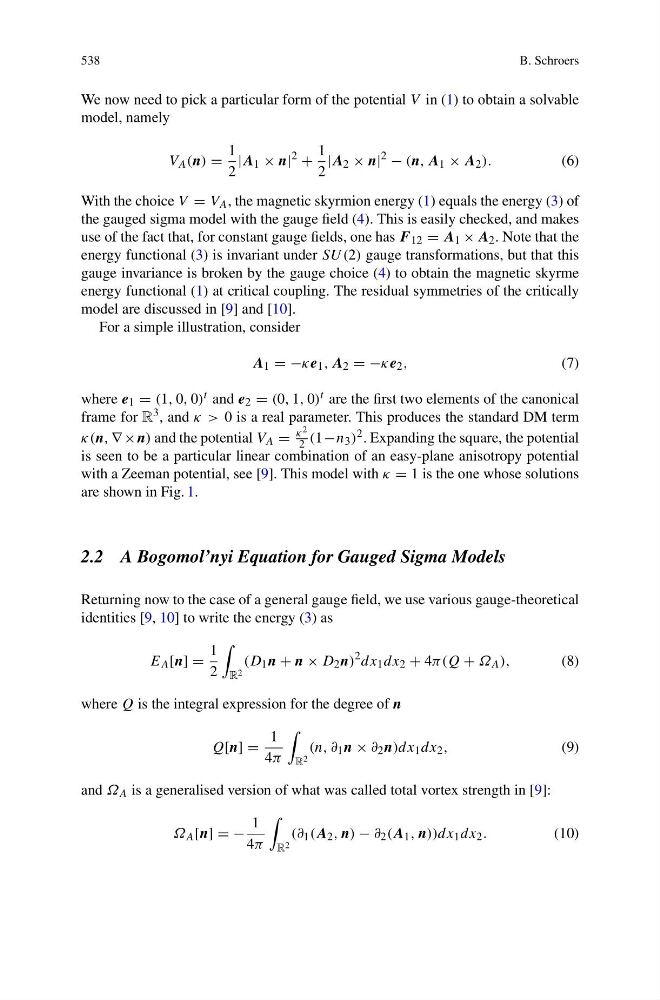
We now need to pick a particular form of the potential V in (1) to obtain a solvable
model, namely
V A (n) =
1
2
|A 1 × n|
2
+
1
2
|A 2 × n|
2
− (n, A 1 × A 2 ).
(6)
With the choice V = V A , the magnetic skyrmion energy (1) equals the energy (3) of
the gauged sigma model with the gauge field (4). This is easily checked, and makes
use of the fact that, for constant gauge fields, one has F 12 = A 1 × A 2 . Note that the
energy functional (3) is invariant under SU (2) gauge transformations, but that this
gauge invariance is broken by the gauge choice (4) to obtain the magnetic skyrme
energy functional (1) at critical coupling. The residual symmetries of the critically
model are discussed in [9] and [10].
For a simple illustration, consider
A 1 = −κe 1 , A 2 = −κe 2 ,
(7)
where e 1 = (1, 0, 0) t and e 2 = (0, 1, 0) t are the first two elements of the canonical
frame for R 3 , and κ > 0 is a real parameter. This produces the standard DM term
κ(n, ∇ ×n) and the potential V A =
κ 2
2 (1−n 3 ) 2 . Expanding the square, the potential
is seen to be a particular linear combination of an easy-plane anisotropy potential
with a Zeeman potential, see [9]. This model with κ = 1 is the one whose solutions
are shown in Fig. 1.
2.2 A Bogomol’nyi Equation for Gauged Sigma Models
Returning now to the case of a general gauge field, we use various gauge-theoretical
identities [9, 10] to write the energy (3) as
E A [n] =
1
2
R 2
(D 1 n + n × D 2 n)
2 dx 1 dx 2 + 4π(Q + Ω A ),
(8)
where Q is the integral expression for the degree of n
Q[n] =
1
4π
R 2
(n, ∂ 1 n × ∂ 2 n)dx 1 dx 2 ,
(9)
and Ω A is a generalised version of what was called total vortex strength in [9]:
Ω A [n] = −
1
4π
R 2
(∂ 1 (A 2 , n) − ∂ 2 (A 1 , n))dx 1 dx 2 .
(10)
B. Schroers
We now need to pick a particular form of the potential V in (1) to obtain a solvable
model, namely
V A (n) =
1
2
|A 1 × n|
2
+
1
2
|A 2 × n|
2
− (n, A 1 × A 2 ).
(6)
With the choice V = V A , the magnetic skyrmion energy (1) equals the energy (3) of
the gauged sigma model with the gauge field (4). This is easily checked, and makes
use of the fact that, for constant gauge fields, one has F 12 = A 1 × A 2 . Note that the
energy functional (3) is invariant under SU (2) gauge transformations, but that this
gauge invariance is broken by the gauge choice (4) to obtain the magnetic skyrme
energy functional (1) at critical coupling. The residual symmetries of the critically
model are discussed in [9] and [10].
For a simple illustration, consider
A 1 = −κe 1 , A 2 = −κe 2 ,
(7)
where e 1 = (1, 0, 0) t and e 2 = (0, 1, 0) t are the first two elements of the canonical
frame for R 3 , and κ > 0 is a real parameter. This produces the standard DM term
κ(n, ∇ ×n) and the potential V A =
κ 2
2 (1−n 3 ) 2 . Expanding the square, the potential
is seen to be a particular linear combination of an easy-plane anisotropy potential
with a Zeeman potential, see [9]. This model with κ = 1 is the one whose solutions
are shown in Fig. 1.
2.2 A Bogomol’nyi Equation for Gauged Sigma Models
Returning now to the case of a general gauge field, we use various gauge-theoretical
identities [9, 10] to write the energy (3) as
E A [n] =
1
2
R 2
(D 1 n + n × D 2 n)
2 dx 1 dx 2 + 4π(Q + Ω A ),
(8)
where Q is the integral expression for the degree of n
Q[n] =
1
4π
R 2
(n, ∂ 1 n × ∂ 2 n)dx 1 dx 2 ,
(9)
and Ω A is a generalised version of what was called total vortex strength in [9]:
Ω A [n] = −
1
4π
R 2
(∂ 1 (A 2 , n) − ∂ 2 (A 1 , n))dx 1 dx 2 .
(10)