

536
B. Schroers
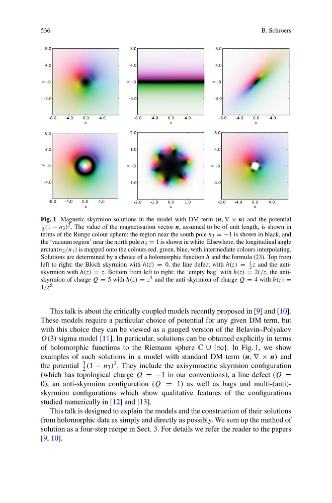
Fig. 1 Magnetic skyrmion solutions in the model with DM term (n, ∇ × n) and the potential
1
2 (1 − n 3 ) 2 . The value of the magnetisation vector n, assumed to be of unit length, is shown in
terms of the Runge colour sphere: the region near the south pole n 3 = −1 is shown in black, and
the ‘vacuum region’ near the north pole n 3 = 1 is shown in white. Elsewhere, the longitudinal angle
arctan(n 2 /n 1 ) is mapped onto the colours red, green, blue, with intermediate colours interpolating.
Solutions are determined by a choice of a holomorphic function h and the formula (23). Top from
left to right: the Bloch skyrmion with h(z) = 0, the line defect with h(z) =
i
2 z and the antiskyrmion with h(z) = z. Bottom from left to right: the ‘empty bag’ with h(z) = 2i/z, the antiskyrmion of charge Q = 5 with h(z) = z 5 and the anti-skyrmion of charge Q = 4 with h(z) =
1/z 5
This talk is about the critically coupled models recently proposed in [9] and [10].
These models require a particular choice of potential for any given DM term, but
with this choice they can be viewed as a gauged version of the Belavin–Polyakov
O(3) sigma model [11]. In particular, solutions can be obtained explicitly in terms
of holomorphic functions to the Riemann sphere C ∪ {∞}. In Fig. 1, we show
examples of such solutions in a model with standard DM term (n, ∇ × n) and
the potential
1
2 (1 − n 3 ) 2 . They include the axisymmetric skyrmion configuration
(which has topological charge Q = −1 in our conventions), a line defect (Q =
0), an anti-skyrmion configuration (Q = 1) as well as bags and multi-(anti)skyrmion configurations which show qualitative features of the configurations
studied numerically in [12] and [13].
This talk is designed to explain the models and the construction of their solutions
from holomorphic data as simply and directly as possibly. We sum up the method of
solution as a four-step recipe in Sect. 3. For details we refer the reader to the papers
[9, 10].
B. Schroers
Fig. 1 Magnetic skyrmion solutions in the model with DM term (n, ∇ × n) and the potential
1
2 (1 − n 3 ) 2 . The value of the magnetisation vector n, assumed to be of unit length, is shown in
terms of the Runge colour sphere: the region near the south pole n 3 = −1 is shown in black, and
the ‘vacuum region’ near the north pole n 3 = 1 is shown in white. Elsewhere, the longitudinal angle
arctan(n 2 /n 1 ) is mapped onto the colours red, green, blue, with intermediate colours interpolating.
Solutions are determined by a choice of a holomorphic function h and the formula (23). Top from
left to right: the Bloch skyrmion with h(z) = 0, the line defect with h(z) =
i
2 z and the antiskyrmion with h(z) = z. Bottom from left to right: the ‘empty bag’ with h(z) = 2i/z, the antiskyrmion of charge Q = 5 with h(z) = z 5 and the anti-skyrmion of charge Q = 4 with h(z) =
1/z 5
This talk is about the critically coupled models recently proposed in [9] and [10].
These models require a particular choice of potential for any given DM term, but
with this choice they can be viewed as a gauged version of the Belavin–Polyakov
O(3) sigma model [11]. In particular, solutions can be obtained explicitly in terms
of holomorphic functions to the Riemann sphere C ∪ {∞}. In Fig. 1, we show
examples of such solutions in a model with standard DM term (n, ∇ × n) and
the potential
1
2 (1 − n 3 ) 2 . They include the axisymmetric skyrmion configuration
(which has topological charge Q = −1 in our conventions), a line defect (Q =
0), an anti-skyrmion configuration (Q = 1) as well as bags and multi-(anti)skyrmion configurations which show qualitative features of the configurations
studied numerically in [12] and [13].
This talk is designed to explain the models and the construction of their solutions
from holomorphic data as simply and directly as possibly. We sum up the method of
solution as a four-step recipe in Sect. 3. For details we refer the reader to the papers
[9, 10].